Ngoc Tran

This page is a cumulative notes of mine and can be used as a quick reference of basic definitions in maths that I often encounter on daily basis.

Table of Contents

• Geometric series
• Power series
• Taylor series
• Gradient
• Scalar product
• Vector Norm
• Cauchy-Schwarz inequality
• Law of Cosine
• Orthogonal vectors
• Projection of a vector on a line
• Normalized vector
• Orthonormal vectors
• Orthogonal matrix
• Span the space
• Four fundamental subspaces
• Singular matrices
• Eigenvalues and Eigenvectors
• Matrix rank
• The Gram-Schmidt process
• Linear independence
• Basis for a space
• Orthogonal
• Projection
• Matrix factorisation
  • 1. Factorisation $A = QR$
  • 2. Factorisation $A = LU$
  • 3. Factorisation $A = S \Lambda S^{-1}$
  • 4. Factorisation $A = Q \Lambda Q^T$
  • 5. Factorisation $A = Q_1 \Sigma Q_2^T$

Geometric series

Geometric series is a special series where there is a constant ratio between two successive terms. The geometric series can be written in the form,

where $a$ is a constant. Note that, $S$ is convergent i.i.f $|r| \lt 1$

References :

1. http://www.sosmath.com/calculus/geoser/geoser01.html
2. https://en.wikipedia.org/wiki/Geometric_series

Power series

The power series is a series in form of,

where $a_n$ is a coefficient of $x_n$, $c$ is a constant

References :

1. http://tutorial.math.lamar.edu/Classes/CalcII/PowerSeriesandFunctions.aspx
2. https://en.wikipedia.org/wiki/Power_series

Taylor series

Taylor series is a series expansion of a function about a point, i.e., a function $f(x)$ can be approximated about a point $x = a$ by using Taylor series.

If $f(x)$ is differential in $(-\infty, +\infty)$, the Taylor expansion of $f(x)$ about a point $x = a$ has a form,

where $f^{(n)}(x)$ is n-th derivative of $f(x)$, e.g., $f^{(1)}(x) = f’(x)$, $f^{(2)}(x) = f’‘(x)$.

References:

1. https://en.wikipedia.org/wiki/Taylor_series
2. http://tutorial.math.lamar.edu/Classes/DE/TaylorSeries.aspx
3. http://davidlowryduda.com/an-intuitive-overview-of-taylor-series/

Gradient

The gradient vector $\nabla f$ of a function $f(x_1, x_2, …, x_n)$ is denoted as,

Simply speaking, $\nabla f$ is simply a vector of partial derivatives of $f$.

References:

1. http://mathworld.wolfram.com/Gradient.html
2. https://goo.gl/C5jBBs

Scalar product

The scalar product (also known as dot product, inner product) of two vectors $x = [x_1, x_2, …, x_n]$ and $y = [y_1, y_2, …, y_n]$ is defined as

Another way to calculate the scalar product of two vectors $x,y$ is

where $\theta$ is the angle between $x,y$.

Note that scalar product is different to scalar multiplication.

Alternatively, using R we can have,

> x
[1] 1 2 3
> y
[1] 4 5 6
> sum(x*y)
[1] 32

References:

1. http://livebooklabs.com/keeppies/c5a5868ce26b8125/73a4ae787085d554
2. http://www.purplemath.com/modules/mtrxmult.htm

Vector Norm

Intuitively speaking, norm of a vector $x = [x_1, x_2, …, x_n]$ is the length of the vector in the space. Norm of the vector $x$ is denoted as $\lVert x \rVert$.

In middle school, the definition of $\lVert x \rVert$ is constraint within the formula $\lVert x \rVert = \sqrt{x_1^2 + x_2^2 + … + x_n^2}$. However, indeed there are numerous ways to calculate the norm and that formula is just one of them.

The norm is universally called as $l_p-norm$. The $l_p-norm$ of $x$ is defined as,

• Given $p = 2$, we will have $l_2-norm$, which is also known as Euclidean norm. Specifically, we have,

• Given $p=3$, we will have $l_3-norm$, which is, \(\lVert x \rVert_3 = \sqrt[3]{\sum_{i=1}^{n} |x_i|^3} = \sqrt[3]{x_1^3 + x_2^3 + ... + x_n^3}\)

Alternatively, using R, we can have,

> x <- as.matrix(c(3,4,5))
> x
     [,1]
[1,]    3
[2,]    4
[3,]    5
> norm(x, "F") #"F" for Euclidean form
[1] 7.071068

References:

1. https://rorasa.wordpress.com/2012/05/13/l0-norm-l1-norm-l2-norm-l-infinity-norm/
2. https://en.wikipedia.org/wiki/Norm_(mathematics)

Cauchy-Schwarz inequality

For any two vectors $x, y \in \mathbb{R}^n$, we have,

References:

1. http://livebooklabs.com/keeppies/c5a5868ce26b8125/73a4ae787085d554
2. https://en.wikipedia.org/wiki/Cauchy%E2%80%93Schwarz_inequality

Law of Cosine

The law of cosine (or cosine law) is defined as follows.

Given three vectors $x, y, z \in \mathbb{R}^n$, we have

where $\theta$ is the angle between vectors $x, y$.

References:

1. https://www.mathsisfun.com/algebra/trig-cosine-law.html

Orthogonal vectors

Given two vectors $x, y \in \mathbb{R}^n$, $x,y$ are orthogonal i.i.f the scalar product of $x,y$ equals 0. Mathematically, we have,

Projection of a vector on a line

The explanation is given in this video.

References:

1. https://www.khanacademy.org/math/linear-algebra/matrix-transformations/lin-trans-examples/v/expressing-a-projection-on-to-a-line-as-a-matrix-vector-prod

Normalized vector

The normalized vector (or unit vector) $\hat{x}$ of the vector $x \in \mathbb{R}^n$ is a vector whose norm equals to 1 and has the same direction with $x$. Mathematically, we have,

By using R, we can have,

> x <- c(1,2,3,4,5,6)
> x
[1] 1 2 3 4 5 6
> x / sqrt(sum(x^2)) # Using Euclidean norm
[1] 0.1048285 0.2096570 0.3144855 0.4193139 0.5241424
[6] 0.6289709

References:

1. http://mathworld.wolfram.com/UnitVector.html

Orthonormal vectors

Two vectors $q_1, q_2 \in \mathbb{R}^n$ are orthonormal if they are:

1. Unit vectors (or normalized vectors), e.g., $q_1 = \frac{x}{\lVert x \rVert_p}$, and $q_2 = \frac{y}{\lVert y \rVert_p}$ .
2. Orthogonal, e.g., $q_1^Tq_2 = 0$.

By using R, we can have,

> x <- c(1,2,3,4)
> x
[1] 1 2 3 4
> y <- c(3,2,3,-4)
> y
[1]  3  2  3 -4
> x%*%y #vectors x, y are orthogonal
     [,1]
[1,]    0
> x_hat <- x/sqrt(sum(x^2)) #unit vector of x
> x_hat
[1] 0.1825742 0.3651484 0.5477226 0.7302967
> y_hat <- y/sqrt(sum(y^2)) #unit vector of y
> y_hat
[1]  0.4866643  0.3244428  0.4866643 -0.6488857
> x_hat%*%y_hat #x_hat, y_hat are orthonormal vectors
             [,1]
[1,] 5.551115e-17

References:

1. http://mathworld.wolfram.com/OrthonormalVectors.html

Orthogonal matrix

An orthogonal matrix $Q$ is simply a square matrix with orthonormal columns. Mathematically, we have,

where $q_i$ is orthonormal vector.

Note that $Q^TQ = I$

> x <- c(0,0,1)
> y <- c(1,0,0)
> z <- (0,1,0)
> x%*%y #vectors x,y are orthonormal
     [,1]
[1,]    0
> x%*%z #vectors x,z are orthonormal
     [,1]
[1,]    0
> y%*%z #vectors y,z are orthonormal
     [,1]
[1,]    0
> Q <- matrix(c(x,y,z), nrow = 3, byrow = FALSE) #Q is orthogonal matrix
> Q #Q is a permutation matrix
     [,1] [,2] [,3]
[1,]    0    1    0
[2,]    0    0    1
[3,]    1    0    0
> t(Q) #transpose of Q
     [,1] [,2] [,3]
[1,]    0    0    1
[2,]    1    0    0
[3,]    0    1    0
> Q%*%t(Q) #Q^T*Q = I
     [,1] [,2] [,3]
[1,]    1    0    0
[2,]    0    1    0
[3,]    0    0    1

References:

1. Linear Algebra and Its Application, Gilbert Strang, 3rd Edition.

Span the space

Vectors $v_1, …, v_n$ span a space $V$ means that the space consists of all combinations of these vectors. Another way to understand is that __we can express any random vector $w$ in the vector space $V$ by a linear combination of the vectors $v_i$, e.g., $w = c_1v_1 + c_2v_2 + … + c_nv_n$.

Mathematically, we have the definition of span.

References:

1. https://www.khanacademy.org/math/linear-algebra/vectors-and-spaces/linear-combinations/v/linear-combinations-and-span

Four fundamental subspaces

There are four fundamental subspaces of a matrix

1. The column space of the matrix $A$, denoted by $C(A)$ The column space of a matrix is defined by the span of all column vectors $c_i$.

where $c_i \in \mathbb{R}^{mxn}$ is the column vectors of the matrix $A$, $w_i \in \mathbb{R}$ is the coefficients.

• The nullspace of the matrix $A$, denoted by $N(A)$ The null space of a matrix contains all vectors $x$ such that $Ax = 0$.

• The row space of the matrix $A$, denoted by $R(A)$ The row space $R(A)$ is the column space of $A^T$. Thus, $R(A) = C(A^T)$.
• The left nullspace of the matrix $A$ The left null space of $A$ is the nullspace of $A^T$.

Example:

Suppose we have the matrix \(A = \begin{bmatrix} 1 & 1 & 1 & 1 \\ 1 & 2 & 3 & 4 \\ 4 & 3 & 2 & 1 \end{bmatrix}\), we have,

1.The column space $C(A)$

Let’s say $w_1 = 2, w_2 = 3, w_3 = 1, w_4 = 1$, we have a vector

\(\begin{align} v = 2\begin{bmatrix} 1 \\ 1 \\ 4 \end{bmatrix} + 3\begin{bmatrix} 1 \\ 2 \\ 3 \end{bmatrix} + 1\begin{bmatrix} 1 \\ 3 \\ 2 \end{bmatrix} + 1\begin{bmatrix} 1 \\ 4 \\ 1 \end{bmatrix} = \begin{bmatrix} 7 \\ 15 \\ 20 \end{bmatrix} \end{align}\).

Since $v$ is the result of the linear combination, \(v = \begin{bmatrix} 7 \\ 15 \\ 20 \end{bmatrix}\) is in the column space $C(A)$.

2.The nullspace $N(A)$

Thus,

Finally, we have,

References:

1. Linear algebra and its application, Gilbert Strang, 3rd Edition.
2. https://www.khanacademy.org/math/linear-algebra/vectors-and-spaces/null-column-space/v/null-space-2-calculating-the-null-space-of-a-matrix

Singular matrices

Singular matrix is a square matrix which does not have an inverse. A square matrix is singular iif its determinant is zero.

For example:

is singular since

Geometric interpretation A matrix can be thought of as a linear function from a vector space $V$ to a vector space $W$. Typically, one is concerned with $n×n$ real matrices, which are linear functions from $ℝ^n$ to $ℝ^n$. An $n×n$ real matrix is non-singular if its image as a function is all of $ℝ^n$ and singular otherwise. More intuitively, it is singular if it misses some point in $n$-dimensional space and non-singular if it doesn’t.

References:

1. Linear algebra and its application, Gilbert Strang, 3rd Edition.
2. http://math.stackexchange.com/questions/166021/what-is-the-geometric-meaning-of-singular-matrix

Eigenvalues and Eigenvectors

Suppose we have a matrix $A$ that acts like a function, when it would takes a vector $x$ and output a vector $Ax$. At this moment, we are more interested in vectors that come out in the same direction as they went in. That is not typical and there will be only a few vectors $Ax$ that are parallel to $x$. Those are called eigenvectors. It can be expressed by

where we would call $\lambda$ the eigenvalue and $x$ the eigenvector.

**How to solve $Ax = \lambda x$

Step 1. Rewrite: $(A - \lambda I)x = 0$

We can see that the matrix $A - \lambda I$ must be singular otherwise, $x$ is a zero matrix, which is not interesting at all!

Proof: Suppose the matrix $T = A - \lambda$, thus we have

Multiply both side of the equation by $T^{-1}$, we have

If $T$ is a singular matrix, then

We conclude that if $T$ is singular, then $x = 0$, which is too obvious that it is not interesting at all!

Step 2. Because $A - \lambda I$ is a singular matrix, we would have

By computing the determinant of $A - \lambda I$, we can find the eigenvalue $\lambda$.

Step 3. For each eigenvalue, solve the equation $(A - \lambda I) x = 0$ to find eigenvector $x$.

References:

1. Linear algebra and its application, Gilbert Strang, 3rd Edition.

Matrix rank

The rank of matrix equals to the maximum number of independent columns or the maximum number of independent row.

• Every matrix of rank one has the simple form $A = uv^T$

References:

1. https://en.wikipedia.org/wiki/Rank_(linear_algebra)

The Gram-Schmidt process

The Gram-Schmidt process is a method for orthonormalising a set of vectors.

Linear independence

Vectors $v_1, …, v_k$ are linearly independent if $ c_1 v_1 + … + c_k v_k = 0$ only happens when $c_1 = c_2 = … = c_k = 0$.

If the columns are linearly independent, the nullspace contains only zero vectors.

References:

1. Linear algebra and its application, Gilbert Strang, 3rd Edition.

Basis for a space

Basis for a space is a sequence of vectors $v_1, v_2, …, v_d$ with 2 properties:

1. They are independent.
2. They span the space.

It means that every vector in the space is a combination of the basis vector because basis vectors span the space.

References:

1. Linear algebra and its application, Gilbert Strang, 3rd Edition.

Orthogonal

Subspace $S$ is orthogonal to subspace $T$ means every vector in $S$ is orthogonal to every vector in $T$.

** It is important to remember that a plane cannot be orthogonal to a plan.

A typical example is that the wall and the floor of a room look like perpendicular planes in $\mathbb{R}^3$. But by the definition of algebra, it is not so. Because the common line in both the wall and the floor cannot be orthogonal to itself.

1. The row space is orthogonal to the null space & the column space is orthogonal to the left nullspace.

Proof: Suppose $x$ is the vector in the null space. Thus, we have $Ax = 0$.

It means that we have $row 1 \cdot x = 0$ $\Rightarrow$ row 1 is orthogonal to $x$.

2. The space off all vectors orthogonal to a subspace $V$ is called the orthogonal complement of $V$, and denoted by $V^{\perp}$.

As a result, the row space and the nullspace are orthogonal complements.

Projection

1. The cosine of the angle between any two vectors $a$ and $b$ is

Proof: Using the law of cosine, we have,

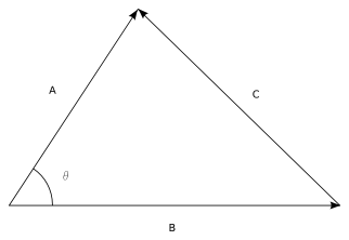
The cosine of the angle between two vectors $a$ and $b$

2. The projection of $b$ onto $a$ is

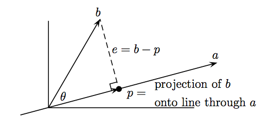
The projection of $b$ onto $a$ where $p = xa$

Proof: we have $p = xa$ (because $p$ is on $a$), thus we have the vector $e = b - p$.

Because $e$ is orthogonal to $a$, we can have $a^Te = 0$.

3. The projection matrix $\mathbf{P}$ is the matrix that project $b$ onto $a$

Proof: We already have in (\ref{projection_matrix}) that $p = \frac{a^Tb}{a^Ta}a$, by rewriting

Matrix factorisation

1. Factorisation $A = QR$

We can factorise any square matrix $A$ as

where $Q$ is an orthogonal matrix, $R$ is an upper triangular matrix.

> x <- matrix(data = c(1, 1, 2, 0, 0, 1, 1, 0, 0), nrow = 3, ncol = 3, byrow = T)
> x
     [,1] [,2] [,3]
[1,]    1    1    2
[2,]    0    0    1
[3,]    1    0    0
> qr(x)
$qr
           [,1]       [,2]      [,3]
[1,] -1.4142136 -0.7071068 -1.414214
[2,]  0.0000000 -0.7071068 -1.414214
[3,]  0.7071068 -1.0000000  1.000000

$rank
[1] 3

$qraux
[1] 1.707107 1.000000 1.000000

$pivot
[1] 1 2 3

attr(,"class")
[1] "qr"

2. Factorisation $A = LU$

LU decomposition simply refers to the transformation of the square matrix $A$ into the product of two different matrices $L$ (lower triangular matrix) and $U$ (upper triangular matrix). Mathematically, we have $A = LU$.

By using R, we can also have,

> library(pracma)
> x <- matrix(c(1, 2, 3, 4, 5, 6, 7, 8, 9), nrow = 3, byrow = TRUE)
> x
     [,1] [,2] [,3]
[1,]    1    2    3
[2,]    4    5    6
[3,]    7    8    9
> lu(x)
$L
     [,1] [,2] [,3]
[1,]    1    0    0
[2,]    4    1    0
[3,]    7    2    1

$U
     [,1] [,2] [,3]
[1,]    1    2    3
[2,]    0   -3   -6
[3,]    0    0    0

3. Factorisation $A = S \Lambda S^{-1}$

Given the eigenvector matrix $S$, which has the form $S = \begin{bmatrix} x_1 & x_2 & \cdots & x_n \end{bmatrix}$, where $x_1, …, x_n$ are the eigenvectors of any square matrix $A$ with distinct eigenvalues $\lambda_1, …, \lambda_n$, we can use $S$ to diagonalise A mathematically by

where $\Lambda$ is the eigenvalue matrix, which has the form \(\Lambda = \begin{bmatrix} \lambda_1 & & & \\ & \lambda_2 & & & \\ \ & & \ddots & \\ & & & \lambda_n \end{bmatrix}\)

From that we can also have

> A <- matrix(data = c(2, 1, 0, 0), nrow = 2, ncol = 2, byrow = T) # Define the matrix
> A
     [,1] [,2]
[1,]    2    1
[2,]    0    0
> E <- eigen(A) # Find eigenvectors and eigenvalues of A
> S <- E$vectors # The eigenvector matrix S
> Lambda <- diag(E$values) # The eigenvalue matrix Lambda
> S_inv <- solve(S)
> A <- S %*% Lambda %*% S_inv # Confirm if A = S*Lambda*S_inv
> A
     [,1] [,2]
[1,]    2    1
[2,]    0    0

4. Factorisation $A = Q \Lambda Q^T$

Given the factorisation $A = S \Lambda S^{-1}$, if matrix $A$ is symmetric, we can have

where $S$ is the eigenvector matrix, $\Lambda$ is the eigenvalue matrix, $Q$ is the orthogonal matrix.

We can see that when $A$ is symmetric, the orthogonal matrix $S$ can be the orthogonal matrix $Q$ (which also mean eigenvectors are orthogonal to each other).

> A <- matrix(data = c(2, -1, -1, 2), nrow = 2, ncol = 2, byrow = T) # Matrix A
> A
     [,1] [,2]
[1,]    2   -1
[2,]   -1    2
> E <- eigen(A) # Find eigenvectors and eigenvalues of A
> S <- E$vectors # The eigenvector matrix S
> Lambda <- diag(E$values) # The eigenvalue matrix Lambda
> S_inv <- solve(S)
> A <- S %*% Lambda %*% S_inv # Confirm if A = S*Lambda*S_inv
> A
     [,1] [,2]
[1,]    2   -1
[2,]   -1    2
> t(S) %*% S # Check if S is orthogonal matrix
              [,1]          [,2]
[1,]  1.000000e+00 -2.237114e-17
[2,] -2.237114e-17  1.000000e+00

5. Factorisation $A = Q_1 \Sigma Q_2^T$

Any $m x n$ matrix $A$ can be factored into

The columns of $Q_1$ ($m$ by $m$) are eigenvectors of $AA^T$, and the columns of $Q_2$ ($n$ by $n$) are eigenvectors of $A^TA$. The $r$ singular values on the diagonal of $\Sigma$ ($m$ by $n$) are the square roots of the nonzero eigenvalues of both $AA^T$ and $A^TA$.

References:

1. https://autarkaw.org/2008/06/04/lu-decomposition-takes-more-computational-time-than-gaussian-elimination-what-gives/
2. http://math.stackexchange.com/questions/266355/necessity-advantage-of-lu-decomposition-over-gaussian-elimination