Table of Contents
- Paired t-test
- Analysis of Variance (ANOVA)
- Chi-squared test
- McNemar’s test
- Sign test
- Wilcoxon signed-rank test
Paired t-test
A paired t-test is used to compare two population means where you have two samples in which observations in one sample can be paired with observations in the other sample. Examples of where this might occur are:
- Before-and-after observations on the same subjects (e.g. students’ diagnostic test results before and after a particular module or course).
- A comparison of two different methods of measurement or two different treatments where the measurements/treatments are applied to the same subjects.
NOTE: For this test to be valid the differences only need to be approximately normally distributed. Therefore, it would not be advisable to use a paired t-test where there were any extreme outliers.
Example:
Suppose a sample of n students were given a diagnostic test before studying a particular module and then again after completing the module. We want to find out if, in general, our teaching leads to improvements in students’ knowledge/skills (i.e. test scores). We can use the results from our sample of students to draw conclusions about the impact of this module in general.
Let x = test score before the module, y = test score after the module. To test the null hypothesis that the true mean difference is zero, the procedure is as follows:
-
Calculate the difference ($d_i = y_i − x_i$) between the two observations on each pair, making sure you distinguish between positive and negative differences.
-
Calculate the mean difference, $\bar{d}$.
-
Calculate the standard deviation of the differences, $s_d$, and use this to calculate the standard error of the mean difference, \(SE(\bar{d}) = \frac{s_d}{\sqrt{n}}\).
-
Calculate the t-statistic, which is given by \(T = \frac{\bar{d}}{SE(d)}\). Under the null hypothesis, this statistic follows a t-distribution with $n − 1$ degrees of freedom.
-
Use tables of the t-distribution to compare your value for $T$ to the $t_{n−1}$ distribution. This will give the p-value for the paired t-test.
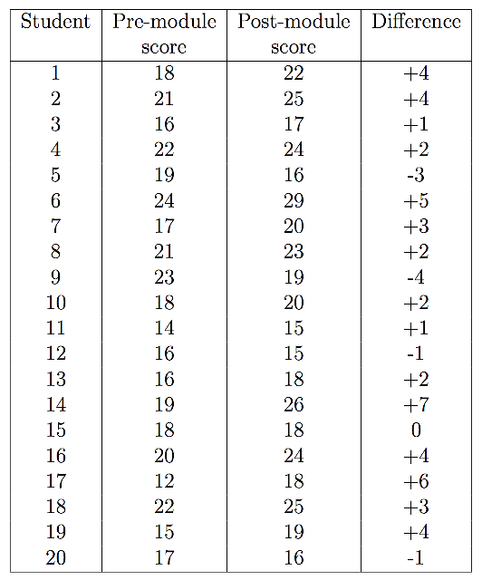
Example data
Calculating the mean and standard deviation of the differences gives: $\bar{d} = 2.05$ and $sd = 2.837$. Therefore, $SE(\bar{d}) = \frac{s_d}{\sqrt{n}} = \frac{2.837}{\sqrt{20}} = 0.634$.
Looking this up in tables gives $p = 0.004$. Therefore, there is strong evidence that, on average, the module does lead to improvements.
> x <- c(18, 21, 16, 22, 19, 24, 17, 21, 23, 18, 14, 16, 16, 19, 18, 20, 12, 22,
+        15, 17)
> y <- c(22, 25, 17, 24, 16, 29, 20, 23, 19, 20, 15, 15, 18, 26, 18, 24, 18, 25,
+        19, 16)
> t.test(x, y, paired = T)

	Paired t-test

data:  x and y
t = -3.2313, df = 19, p-value = 0.004395
alternative hypothesis: true difference in means is not equal to 0
95 percent confidence interval:
 -3.3778749 -0.7221251
sample estimates:
mean of the differences
                  -2.05
Required assumptions for the t-test
-
Normality or pseudo-normality Dataset with $\gt 30$ instances should be sufficient.
-
Randomness of the Samples Instances are randomly chosen from the population.
-
Equal variances of the populations The t-test assumes that the samples come from populations with equal variance. Can be verified by tests such as F test, Bartlett’s test, Levene’s test, or the Brown–Forsythe test.
Analysis of Variance (ANOVA)
ANOVA is a statistical procedure to compare > 2 means.
1. One-way ANOVA
Example:
Test if the amount of caffeine consumed affected memory. The participants were divided into 3 groups randomly (1) Coca-cola classic (34mg), (2) McDonald’s coffee (100mg), and (3) Jolt energy (160mg). After drinking the beverage, the participants were given a memory test - words remembered from a list. The data is in Figure 1.
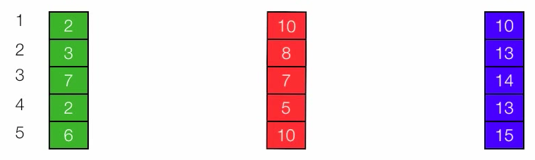
Figure 1. Number of words recalled in memory test
a) Step 1:
- Factor: cafeine.
- Levels: 3.
- Response variable: memory.
- Null hypothesis $H_0$: means among the groups are the same, i.e., $\mu_A = \mu_B = \mu_C$.
- Alternative hypothesis $H_a$: means are not the same.
b) Step 2:
There is 2 components of variation in the number of words remembered by the participants.
- Between-group variation: variation in the number of words recalled among the 3 groups.
- Within-group variation: variation in the number of words among participants of each group.
To measure 2 components, we will compute Sum of Squares within Groups (SSWG) (Figure 2) and Sum of Squares between Groups (SSBG) (Figure 3).
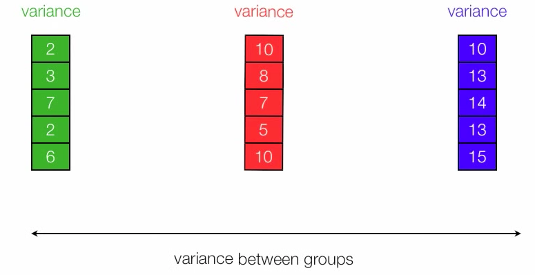
Figure 2. We can measure between-group variation by SSBG
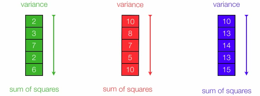
Figure 3. We can measure within-group variation by SSWG
Thus, we have Total Sum of Squares (TSS) = SSWG + SSBG (Figure 4).
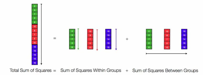
Figure 4. Total Sum of Squares
c) Step 3:
- Compute SSWG.
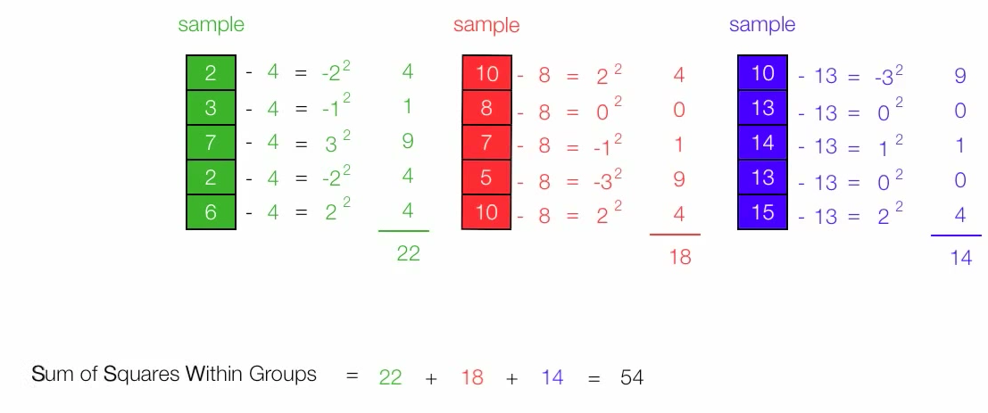
Figure 5. Calculate SSWG. Note that 4, 8 and 13 are means of each group respectively.
- Compute SSBG.
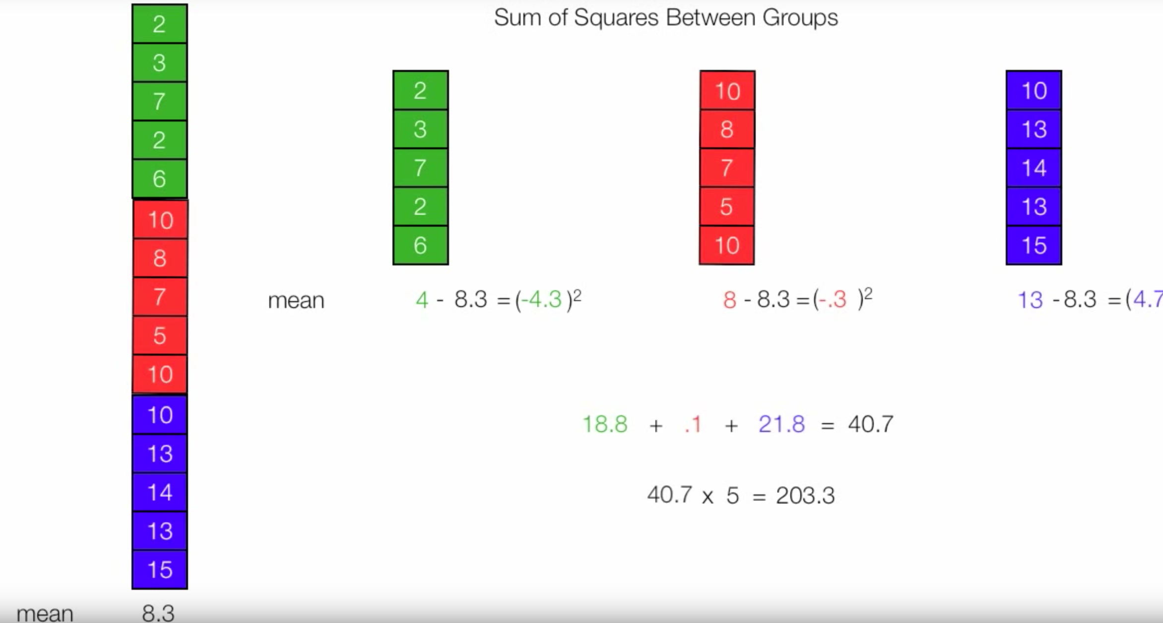
Figure 5. Calculate SSBG. Note that 4, 8 and 13 are means of each group respectively.
- Compute TSS.
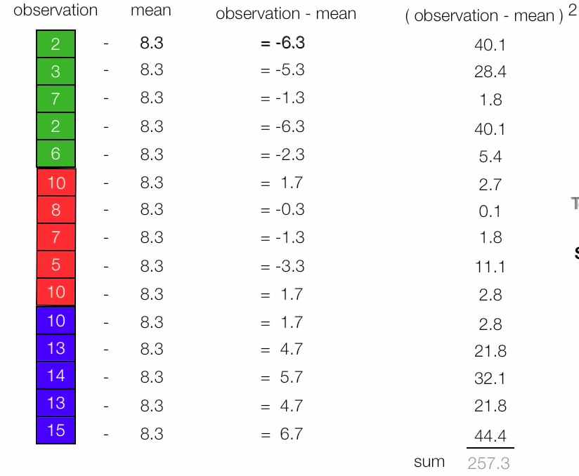
Figure 6. Calculate TSS. Note that 8.3 is the mean of 3 groups together.
d) Step 4:
Calculate $F$ score.
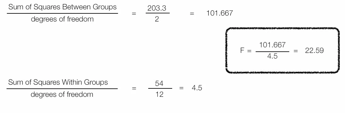
Figure 7. Calculate F-score.
Implementation in R:
> a <- c(2,3,7,2,6)
> b <- c(10, 8, 7, 5, 10)
> c <- c(10, 13, 14, 13, 15)
>
> val <- c(a, b, c)
> cat <- c(rep("A", 5), rep("B", 5), rep("C", 5))
> dt <- data.frame(val, cat)
> rslt <- aov(val ~ cat, data = dt)
> summary(rslt)
            Df Sum Sq Mean Sq F value   Pr(>F)
cat          2  203.3   101.7   22.59 8.54e-05 ***
Residuals   12   54.0     4.5
---
Signif. codes:  0 ‘***’ 0.001 ‘**’ 0.01 ‘*’ 0.05 ‘.’ 0.1 ‘ ’ 1
According to the founded p-value, we reject the null hypothesis $H_0$, which suggests that there are differences among groups. However, it is important to know that ANOVA does not tell which groups differ, only that at least 2 groups among 3 differ.
2. Two-way ANOVA
Use two-way ANOVA when we have 2 factors in the data.
> delivery.df = data.frame(
+   Service = c(rep("Carrier 1", 15), rep("Carrier 2", 15),
+               rep("Carrier 3", 15)),
+   Destination = c(rep(c("Office 1", "Office 2", "Office 3",
+                         "Office 4", "Office 5"), 9)),
+   Time = c(15.23, 14.32, 14.77, 15.12, 14.05,
+            15.48, 14.13, 14.46, 15.62, 14.23, 15.19, 14.67, 14.48, 15.34, 14.22,
+            16.66, 16.27, 16.35, 16.93, 15.05, 16.98, 16.43, 15.95, 16.73, 15.62,
+            16.53, 16.26, 15.69, 16.97, 15.37, 17.12, 16.65, 15.73, 17.77, 15.52,
+            16.15, 16.86, 15.18, 17.96, 15.26, 16.36, 16.44, 14.82, 17.62, 15.04)
+ )
> head(delivery.df)
    Service Destination  Time
1 Carrier 1    Office 1 15.23
2 Carrier 1    Office 2 14.32
3 Carrier 1    Office 3 14.77
4 Carrier 1    Office 4 15.12
5 Carrier 1    Office 5 14.05
6 Carrier 1    Office 1 15.48
> rslt <- aov(Time ~ Service * Destination, data = delivery.df)
> summary(rslt)
                    Df Sum Sq Mean Sq F value   Pr(>F)
Service              2 23.171  11.585 161.560  < 2e-16 ***
Destination          4 17.542   4.385  61.155 5.41e-14 ***
Service:Destination  8  4.189   0.524   7.302 2.36e-05 ***
Residuals           30  2.151   0.072
---
Signif. codes:  0 ‘***’ 0.001 ‘**’ 0.01 ‘*’ 0.05 ‘.’ 0.1 ‘ ’ 1
References:
Chi-squared test
The Chi-squared test is for categorial data to test how likely it is that an observed distribution is due to chance. The test is also known as goodness of fit test, because it measures how well the observed distribution fit the distribution that is expected if the variables are independent.
Example:
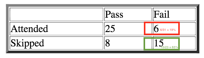
Figure 1. Contingency table of the data
Suppose we wish to determine if there is a relationship between attending the class and passing the course. We will use Chi-squared test to figure out.
What Chi-squared test actually does is making a comparison between the percentage of the red and green percentages, which means comparing the percentage of students who attended the class but still fails, and the percentage of student skipped the class and fail. If those percentages are equal, the chi-squared test statistic is zero. It would mean that there is no relationship between attending the class and failing the course.
In our example, we can see that two percentages are not the same, so we could expect that there is an underlying relationship between two given variables.
- Null hypothesis $H_0$: Passing the class and Attending the course are independent, which implies there is no association between two variables.
- Alternative hypothesis $H_A$: two variables are dependent, which implies there is a relationship between them.
> mtrx <- matrix(c(25, 6, 8, 15), byrow = T, nrow = 2, ncol = 2)
> colnames(mtrx) <- c("Pass", "Fail")
> rownames(mtrx) <- c("Attended", "Skipped")
> tbl <- as.table(mtrx)
> tbl
         Pass Fail
Attended   25    6
Skipped     8   15
> chisq.test(tbl, correct = F)

	Pearson's Chi-squared test

data:  tbl
X-squared = 11.686, df = 1, p-value = 0.0006297
Because p-value « 0.05, we reject the null hypothesis and accept the alternative hypothesis. The outcome of the test suggests that attending the class and passing the course are two dependent variables.
References:
- http://www.ling.upenn.edu/~clight/chisquared.htm
- http://www.theanalysisfactor.com/difference-between-chi-square-test-and-mcnemar-test/
McNemar’s test
McNemar’s test is essentially a paired version of Chi-squared test. We, for example, can use McNemar’s test to test if the number of participants were significantly changed after and before an experiment.
McNemar’s test can only be applied to 2x2 table, rather than larger tables like Chi-squared test. More importantly, unlike Chi-squared test by which we can use to test the independence/dependence between two categorial variables, we use McNemar’s test to test for consistency in response across two variables.
Our example is introduced in Figure 1. We will use McNemar’s test to verify whether or not the treatment is effective. What McNemar’s test essentially does is recognizing if the number of people move from Yes to No and vice versa randomly. To do that, McNemar’s test ignores the number of patients who are consistently Yes and No before and after the treatment. Instead the test steers its focus on the number of patients changing answers. In Figure 1, the focus is purple cells.
Note: we do not use row percentage in McNemar’s test as in Chi-squared test. McNemar’s test directly compares the numbers.
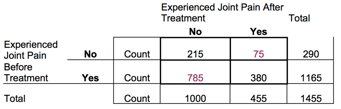
Figure 1
- Null hypothesis $H_0$: The treatment has no effect.
- Alternative hypothesis $H_A$: The treatment has some effects.
> mtrx <- matrix(c(215, 75, 785, 380), byrow = T, nrow = 2, ncol = 2)
> colnames(mtrx) <- c("No", "Yes")
> rownames(mtrx) <- c("No", "Yes")
> tbl <- as.table(mtrx)
> tbl
     No Yes
No  215  75
Yes 785 380
> mcnemar.test(tbl, correct = F)

	McNemar's Chi-squared test

data:  tbl
McNemar's chi-squared = 586.16, df = 1, p-value < 2.2e-16
Because the p-value is $\ll 0.05$, we reject $H_0$ and accept $H_A$, which suggests that there were some effects of the treatment.
References:
- http://www.theanalysisfactor.com/difference-between-chi-square-test-and-mcnemar-test/
- https://en.wikipedia.org/wiki/McNemar%27s_test
- http://yatani.jp/teaching/doku.php?id=hcistats:chisquare
Sign test
The sign test can be used to determine (1) if two groups are equally sized, (2) if the median of a group $lt$, $gt$ a specified value.
Assumptions:
- Normal distribution The sign test is non-parametric, thus, the data does not need to have Gaussian distribution form.
- Independent samples Two samples are independent.
- Dependent samples Two samples should be paired (“before-after” sample)
Example 1: Compare two groups using two independent samples
The table below shows the hours of relief provided by two analgesic drugs in 12 patients suffering from arthritis. Is there any evidence that one drug provides longer relief than the other?
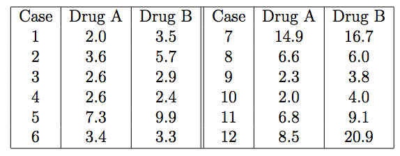
Figure 1
- Null hypothesis $H_0$: Median of hours of relief of group A equals to that of group B, $m_A = m_B$
- Alternative hypothesis $H_A$: $m_A$ is not equal to $m_B$
> library(BSDA)
> x <- c(2.0, 3.6, 2.6, 2.6, 7.3, 3.4, 14.9, 6.6, 2.3, 2.0, 6.8, 8.5)
> y <- c(3.5, 5.7, 2.9, 2.4, 9.9, 3.3, 16.7, 6.0, 3.8, 4.0, 9.1, 20.9)
> SIGN.test(x, y, alternative = "two.side")

	Dependent-samples Sign-Test

data:  x and y
S = 3, p-value = 0.146
alternative hypothesis: true median difference is not equal to 0
95 percent confidence interval:
 -2.27872727  0.05745455
sample estimates:
median of x-y
        -1.65

                  Conf.Level  L.E.pt  U.E.pt
Lower Achieved CI     0.8540 -2.1000 -0.3000
Interpolated CI       0.9500 -2.2787  0.0575
Upper Achieved CI     0.9614 -2.3000  0.1000
Our p-value is $0.146 \gt 0.05$, thus we accept the null hypothesis $H_0$. It suggests that two treatment are not evidently different.
Example 2: Compare the median of a group with a specified value
Recent studies of the private practices of physicians who saw no Medicaid patients suggested that the median length of each patient visit was 22 minutes. It is believed that the median visit length in practices with a large Medicaid load is shorter than 22 minutes. A random sample of 20 visits in practice with a large Medicaid load yielded, in order, the following visit lengths:

Figure 2
Based on these data, is there sufficient evidence to conclude that the median visit length in practices with a large Medicaid load is shorter than 22 minutes?
- Null hypothesis $H_0$: Median of visit length equals to 22 minutes, $m_A = 22$.
- Alternative hypothesis $H_A$: Median of visit length is less than 22”, $m_A < 22$.
> library(BSDA)
> x <- c(9.4, 13.4, 15.6, 16.2, 16.4, 16.8, 18.1, 18.7, 18.9, 19.1, 19.3, 20.1,
+        20.4, 21.6, 21.9, 23.4, 23.5, 24.8, 24.9, 26.8)
> SIGN.test(x, alternative = "less", md = 22)

	One-sample Sign-Test

data:  x
s = 5, p-value = 0.02069
alternative hypothesis: true median is less than 22
95 percent confidence interval:
     -Inf 21.66216
sample estimates:
median of x
       19.2

                  Conf.Level L.E.pt  U.E.pt
Lower Achieved CI     0.9423   -Inf 21.6000
Interpolated CI       0.9500   -Inf 21.6622
Upper Achieved CI     0.9793   -Inf 21.9000
The p-value is $0.0207 \lt 0.05$, which means we reject the null hypothesis $H_0$, and accept the alternative hypothesis. It suggests that the median of visit length is less than 22”.
References:
- http://www.r-tutor.com/elementary-statistics/non-parametric-methods/sign-test
- http://www.statstutor.ac.uk/resources/uploaded/signtest.pdf
- https://onlinecourses.science.psu.edu/stat414/node/318
Wilcoxon signed-rank test
Wilcoxon signed-rank test is a non-parametric test for matched/paired data like the Sign test. However, unlike the Signed test, Wilcoxon signed-rank test takes into account the magnitude of observed differences.
Assumptions:
- Normal distribution Wilcoxon signed-rank test is non-parametric, thus, it does not require the data to be normally distributed.
- Dependent data The test is applicable to dependent data.
- Ordinal/Continuous data type The data has to be measured by using ordinal or continuous level.
Example:
The table below shows the hours of relief provided by two analgesic drugs in 12 patients suffering from arthritis. Is there any evidence that one drug provides longer relief than the other?
Figure 1
- Null hypothesis $H_0$: Median of hours of relief of group A equals to that of group B, $m_A = m_B$
- Alternative hypothesis $H_A$: $m_A$ is not equal to $m_B$
> x <- c(2.0, 3.6, 2.6, 2.6, 7.3, 3.4, 14.9, 6.6, 2.3, 2.0, 6.8, 8.5)
> y <- c(3.5, 5.7, 2.9, 2.4, 9.9, 3.3, 16.7, 6.0, 3.8, 4.0, 9.1, 20.9)
> wilcox.test(x, y, paired = T, alternative = "two.sided", correct = F)

	Wilcoxon signed rank test

data:  x and y
V = 7, p-value = 0.01203
alternative hypothesis: true location shift is not equal to 0

Warning message:
In wilcox.test.default(x, y, paired = T, alternative = "two.sided",  :
  cannot compute exact p-value with ties
References: