I. Introduction

Rough Set (RS) algorithm targets the vagueness of the knowledge, e.g., the boundary between observations is not strong enough to set them apart. Look at Figure 1, we can see that we have no clue how to correctly classify items $x_3$ and $x_4$ when the attribute values of those items are identical.

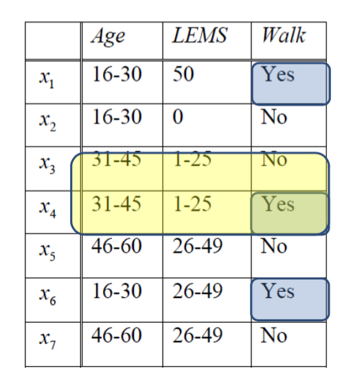
Figure 1: it is impractical to classify x3 and x4

II. Primary concepts of RS

RS theory defines a number of concepts:

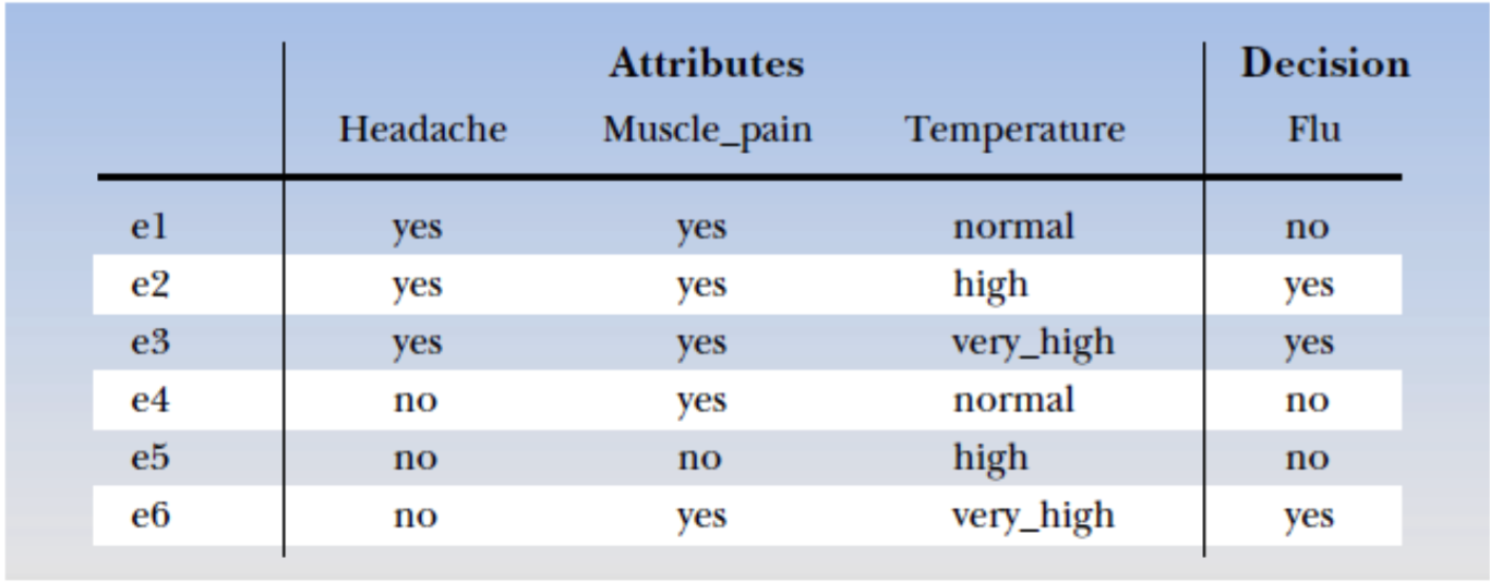
Figure 2: Sample dataset

1) Information system: $I = (U, A)$

Information system can be understood as a body of information/knowledge that we have. Mathematically the information system is denoted as a pair $(U, A)$ where:

• $U = {x_1, x_2, …, x_n}$: universally represents a non-empty $(U \neq \emptyset)$, finite set of observations $x_i$.
• $A = {a_1, a_2, …, a_n}$: represent a non-empty $(A \neq \emptyset)$, finite set of attributes $a_j$ such that $a \in A$, $a: U \rightarrow V_a$, where $V_a$ is the value set of $a$ (which means every observation in $U$ can be set to attributes that belong to $V_a$).

In ML, we usually call $x_i$ observations, objects, rows; and $a_j$ predictors, features, attributes.

2) Decision system: $DS = (U, A \cup {d})$ | $DS \subseteq I$

Decision system $DS$ is a special type of information system $I$ that can be used in classification. $d$ is the decision values (i.e., Yes/No, 1/0, and so on). In ML, we call $d_k \in {d}$ response, or outcome.

3) Indiscernibility relation

Given an information system $I = (U, A)$, for any subset $B \subseteq A$, the indiscernibility or equivalence relation is defined by: \(IND(B) = \{(x, y) \in U^2 | \forall a \in B, a(x) = a(y)\}\) where $IND(B)$ is called the B-indiscernibility relation. The equivalence classes of $IND(B)$ are denoted as $[x]_B$.

Take an example from Figure 2. Suppose we have $B= { Headache, Musclepain }$. Thus, we can have: \(IND(B) = \{\{e1, e2, e3\}, \{e4, e6\}, \{e5\}\}\) We can also say that $e1, e2, e3$ are indiscernible from each other.

4) Approximation

The concept of approximation regards the problem of data reduction in ML. For that, we can define a approximation set $X (X \subseteq U)$ by using the information from the set $B (B \subseteq A)$. To do that, we have to construct $B-lower$ $(\underline{B}X)$ and $B-upper$ $(\overline{B}X)$ approximations of $X$: \(\underline{B}X = \{x | [x]_B \subseteq X\}\) \(\overline{B}X = \{x | [x]_B \cap X \neq \emptyset\}\) Whereas lower-approximation consists of all observations which certainly belong to the class, upper-approximation contains all observations which likely belong to the class.

From that we have $B-boundary$: \(BN_B(X) = \overline{B}X - \underline{B}X\)

and $B-outside$: \(BO_B = U - \overline{B}X\)

Figure 3

For example, in Figure 3, let \(W = \{x | Walk(x) = yes\}\) we can have:

• $\underline{B}W = {x1, x6}$
• $\overline{B}W = {x1, x3, x4, x6}$
• $BN_B(W) = {x3, x4}$
• $BO_B = {x2, x5, x7}$