Table of Contents
In this post, we are going to review classical unconstrained optimization algorithms, including gradient descent, Newton’s and Gauss-Newton. Those three algorithms have been heavily used as optimization methods of different machine learning algorithms, such as linear regression, logistic regression, neural network, and so on.
Note: All R codes of experiments can be found here
1. Gradient descent
1.1. Concept
Gradient descent (or steepest descent) is the most intuitively simple among three algorithms. The underlying mechanism of the algorithm is the concept of the gradient $\nabla$ of the function $f$. Intuitively speaking, $\nabla f$ indicates the direction by which if we traverse along the graph curve of $f$, we are able to find the increasing function values (e.g., $f(x_{n+1}) \gt f(x)$). Conversely, if we traverse the opposite direction of $\nabla f$, we can obtain decreasing values of $f$ such that $f(x_{n+1}) \lt f(x)$. And that’s how gradient descent works!
Mathematically speaking, given a differential function $f(x)$, if
\[x_{n+1} = x_n - \eta \nabla f(x)\]where $\eta$ ($0 \lt \eta < 1$) is the learning rate, $\nabla f(x)$ is the gradient of $f$ at $x_n$.
then,
\[f(x_{n+1}) \geq f(x_n)\]This process stops either after $m$ predefined iterations or until $f(x_{n+1}) \approx f(x_n)$.
1.2. Experiments
Example 1:
Consider $f(x)$ as a quadratic function. Suppose we have $f(x) = ax^2 + bx + c$ with $a = 1, b = 2, c = 3$. We aim to find a value $x^*$ at which we reach the minima of $f(x)$.At the beginning, we blindly set $x_0 = 45$, and sequentially change $\eta = (0.1, 0.3, 0.5, 0.7)$ to observe how the learning rate affects the convergence of the algorithm. Look at Figure 1, at $\eta = 0.1$ (the top left), gradient descent can find the minima of $f(x)$ after roughly 10 iterations. However, from the figure, we can also see that the rate of convergence of the algorithm significantly reduces as soon as it is close to the minima. When $\eta = 0.3$ (the top right), we need roughly 5 iterations, and it seems like at $\eta = 0.5$ (the bottom left), we only need 2 iterations, which is really computationally effective. The worst case is when $\eta = 0.7$ (the bottom right), we “jump” over the minima several times before we approach it.
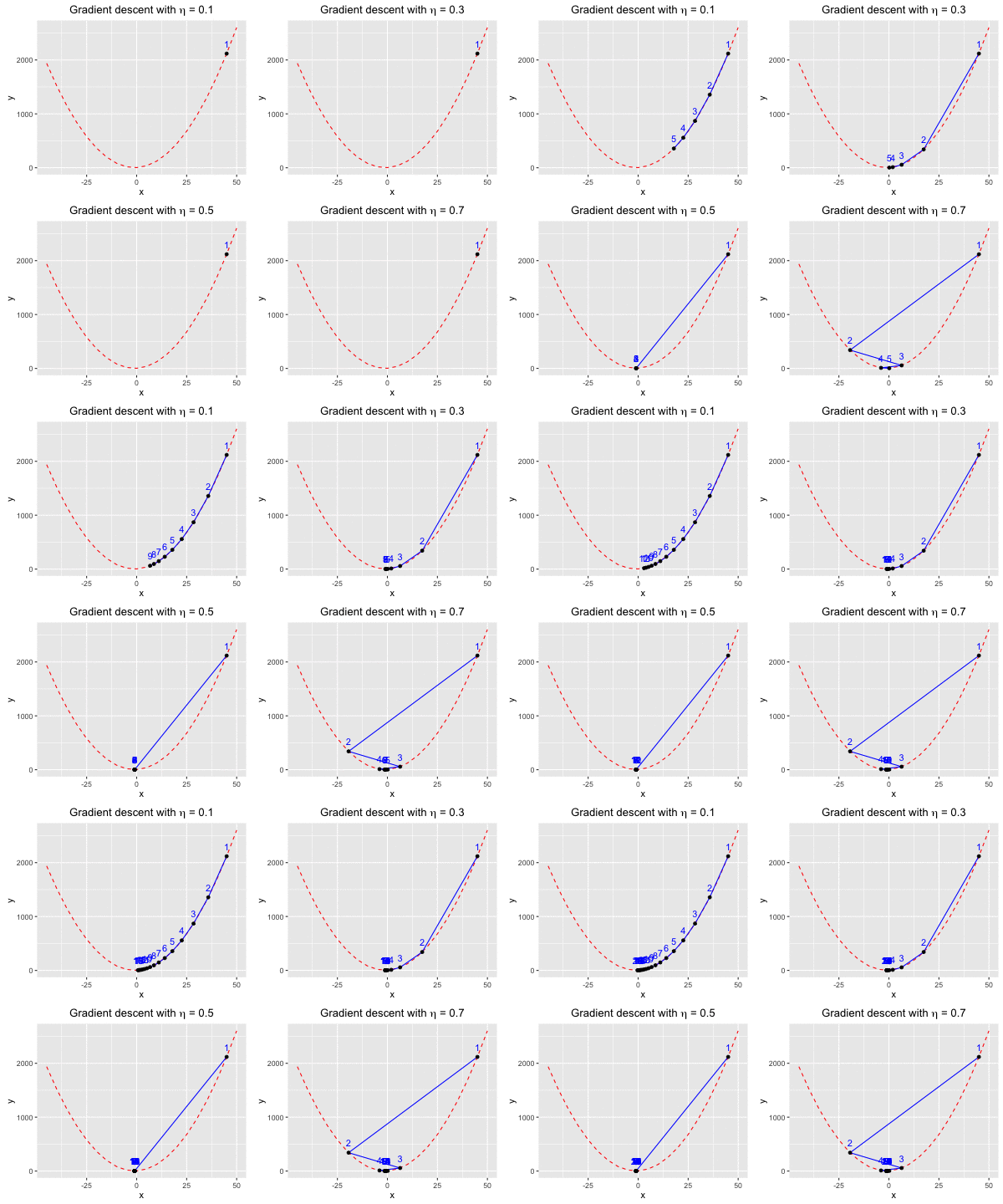
Fig 1. Find the local minima of a quadratic function
Example 2:
Consider $f(x)$ as a polynomial function. Suppose we have $f(x) = -120*x - 154x^2 + 49x^3 + 140x^4 + 70x^5 + 14x^6 + x^7$. We aim to find a value $x^*$ at which we reach the minima of $f(x)$.This example demonstrates that gradient descent cannot guarantee finding global minima of the function although we keep changing $\eta$. The worst case happens when $\eta = 0.02$ (the top right), gradient descent can only find the sub minimal value of the function.
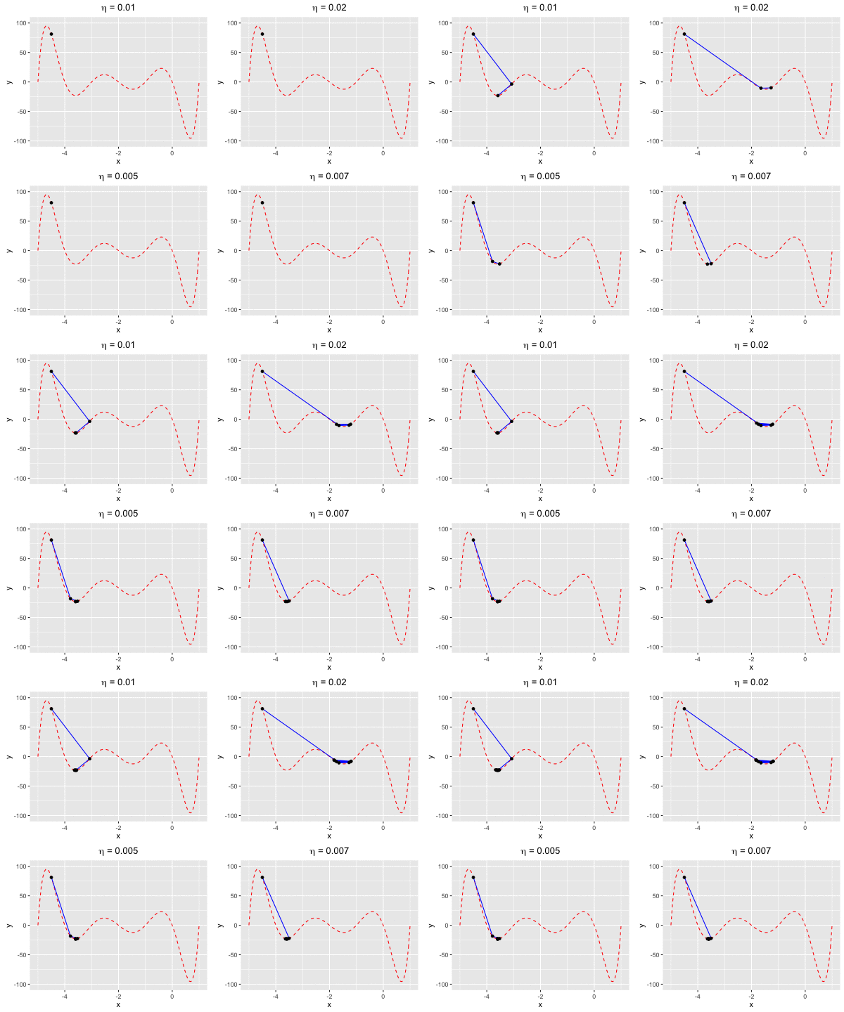
Fig 2. Find the local minima of a polynomial function
2. Newton’s method
2.1. Concept
In my opinion, Newton’s method (or Newton-Raphson method) can be intuitively comprehended as a method to approximate an approximation. It means that if we already have a reasonably good approximation of a function $f$ at a certain value $x_0$, we still can have a better approximation by estimating an approximation of the approximation itself.
I found this page has a brilliant explanation for the algorithm and thus I will reiterate that explanation by my own words.
Suppose we have a function $f(x) \in \mathbb{R^2}$, and we want to find the value of $f$ at a certain value $x_0$. One can say that we can simply plug $x_0$ into $f$ to get the searching value. However, there exist many functions, such as $f = \sqrt{x}$, where we cannot straightforwardly get the value. One can also say that computers can do that. But unlike simple equation like $f(x) = 2x$, where we can compute manually, we do not have any exact expression to describe that root function. In fact, computers use approximation methods behind the scene (like Newton’s method) to compute root value of numbers.
Suppose we want to find an approximation of $f(x^*) = 0$. We do that as follows.
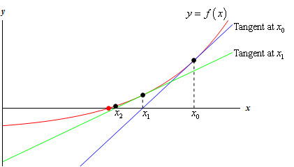
Fig 3. Using 2nd tangent line to have a better approximation
- First, we construct a tangent line (the blue line) at a point $x_0$ where $x_0$ is a guessing point and is reasonably close to the target point where $y = 0$. We can construct the tangent line by using slope-point form. We can see that $x_1$ is a better approximation than $x_0$. However, we are still able to get a better one.
- Second, we construct a second tangent line at $x_1$ (the green line). Again, by using the slope-point form of the tangent line, we have,
- As a result, we can find a closer point $x_1$ by using the formula $x_1 = x_0 - \frac{f(x_0)}{f’{x_0}}$.
2.2. Minimization and maximization problem
Similar to gradient descent, Newton’s method can be used to find optimize the function by setting the derivative to 0 like we explained above.
2.2. Experiments
Example 1:
Consider $f(x)$ as a polynomial function. Suppose we have $f(x) = -120*x - 154x^2 + 49x^3 + 140x^4 + 70x^5 + 14x^6 + x^7$. We aim to find a value $x^*$ at which we reach the minima of $f(x)$.In this example, we are going to find the local minima of $f(x)$ by using both gradient descent and Newton’s method. We can see that the rate of convergence of Newton’s method is higher than gradient descent. This happens due to the fact the Newton’s method makes use of the 2nd-order derivative of $f$.
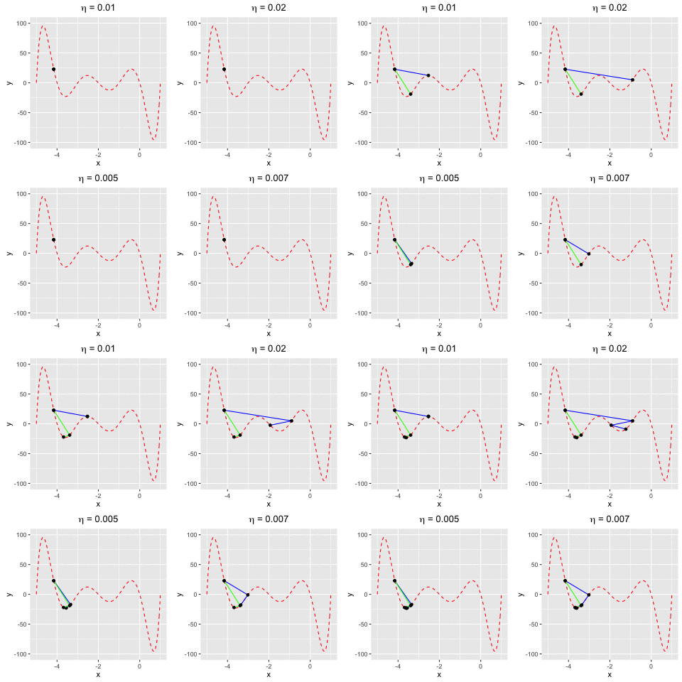
Fig 4. Find the local minima of a polynomial function using both gradient descent and Newton's method
3. Gauss-Newton method
3.1. Concept
Unlike gradient descent and Newton method, Gauss-Newton method can only be used to minimize the sum of squares, such as $C = \frac{1}{2} \sum_{i=1}^{n} (\hat{y}_i - y_i)^2$ where $\hat{y}$ is the predicted output, $y$ is the actual output and $n$ is the total number of observations in the dataset.
Let’s set $e = (\hat{y}_i - y_i)$ , and suppose ${\theta}_j$ is the coefficient vector of the hypothesis function \(h_\theta(x)\) in the $j^{th}$ iteration. For the \((j+1)^{th}\) iteration, the updated error term \(e_{j+1}\) would be,
\[e_{j+1} = e_j + \begin{bmatrix}\frac{\partial e}{\partial \theta}\end{bmatrix}_{\theta = \theta_j}(\theta_{j+1} - \theta_j) \qquad (I)\]We can make (I) more beautiful by employing the concept of Jacobian matrix $J$ such that,
\[J = \begin{bmatrix}\frac{\partial f}{\partial x_1} & \frac{\partial f}{\partial x_2} & \dots & \frac{\partial f}{\partial x_n} \end{bmatrix}\]Thus, we have,
\[(I) \Longleftrightarrow e_{j+1} = e_j + J(\theta_{j+1} - \theta_j) \qquad (II)\]Our goal is finding $\theta_{j+1}$ such that the error term \(e_{j+1}\) is minimal. Mathematically, we have,
\[\theta_{j+1} = \underset{\theta}argmin(\frac{1}{2}\lVert e_{j+1} \rVert_2^2) \qquad (III)\]Remember that \(\lVert v \rVert_2\) is the $l_2$-norm or Euclidiean norm of the vector $v$.
We now need to elaborate \(\lVert e_{j+1} \rVert^2\). First, remember that the norm of a vector $v$ can be defined as \(\lVert v \rVert^2 = v^Tv\). Second, from the equation (II), suppose that,
\[\begin{align} & A = e_j \\ & B = J(\theta_{j+1} - \theta_j) \\ & C = e_{j+1} \end{align}\]Thus, \((II) \Longleftrightarrow C = A + B\). From that, we also have,
\[\begin{align} \lVert C \rVert^2 & = C^TC \\ & = (A + B)^T(A+B) \\ & = (A^T + B^T)(A+B) \\ & = A^TA + A^TB + B^TA + B^TB \end{align}\]Because \(A^TB = \sum a_jb_j = \sum b_ja_j = B^TA\), we can rewrite,
\[C = \lVert A \rVert^2 + 2A^TB + \lVert B \rVert^2 \qquad (IV)\]From (II) and (IV), we can have,
\[\lVert e_{j+1} \rVert^2 = \lVert e_{j} \rVert^2 + 2e^TJ(\theta_{j+1} - \theta_j) + (\theta_{j+1} - \theta_j)^TJ^TJ(\theta_{j+1} - \theta_j) \qquad (V)\]Now, we are going to minimize (V). First, we need to take the derivative of (V) w.r.t. $\theta$ and set it equal to 0, and then find $\theta$. We have
\[\begin{align} & \frac{\partial V}{\partial \theta} = J^Te + J^TJ(\theta_{j+1} - \theta_j) = 0 \\ \Longleftrightarrow & J^TJ(\theta_{j+1} - \theta_j) = -J^Te \\ \Longleftrightarrow & \theta_{j+1} - \theta_j = -(J^TJ)^{-1}J^Te \\ \Longleftrightarrow & \theta_{j+1} = \theta - (J^TJ)^{-1}J^Te \\ \end{align}\]The formula \(\theta_{j+1} = \theta - (J^TJ)^{-1}J^Te\) is the pure form of Gauss-Newton method. By using this equation, we can update the coefficient \(\theta_{j+1}\). To do that, all we need to do is to find the Jacobian matrix. Note that the Gass-Newton method always converge because the Gauss-Newton methods assumes that \(J^TJ\) is non-singular matrix, making it possible to find the inverse matrix.
3.2. Experiments
Example 1:
Suppose we have $f(x) = -120*x - 154x^2 + 49x^3 + 140x^4 + 70x^5 + 14x^6 + x^7$. We first will use $f(x)$ to generate sample data points and second, we will use Gauss-Newton method to fit a model to the generated data points.In Figure 5, we can see that at the beginning, we naively set $\theta =$ [1 1 1 1 1 1 1 1]. In the second iteration, $\theta$ is updated by Gauss-Newton method, allowing the model to fit to the generated data points.
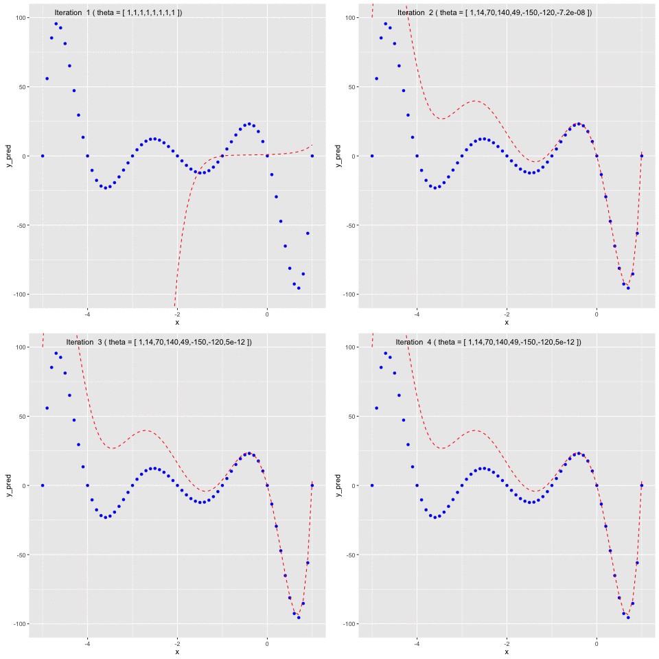
Fig 5. Use Gauss-Newton method to fit generated data points of $f(x)$
Example 2:
Using the dataset Speed and Stopping Distances of Cars, we will find a model that find the relationship between speed and distance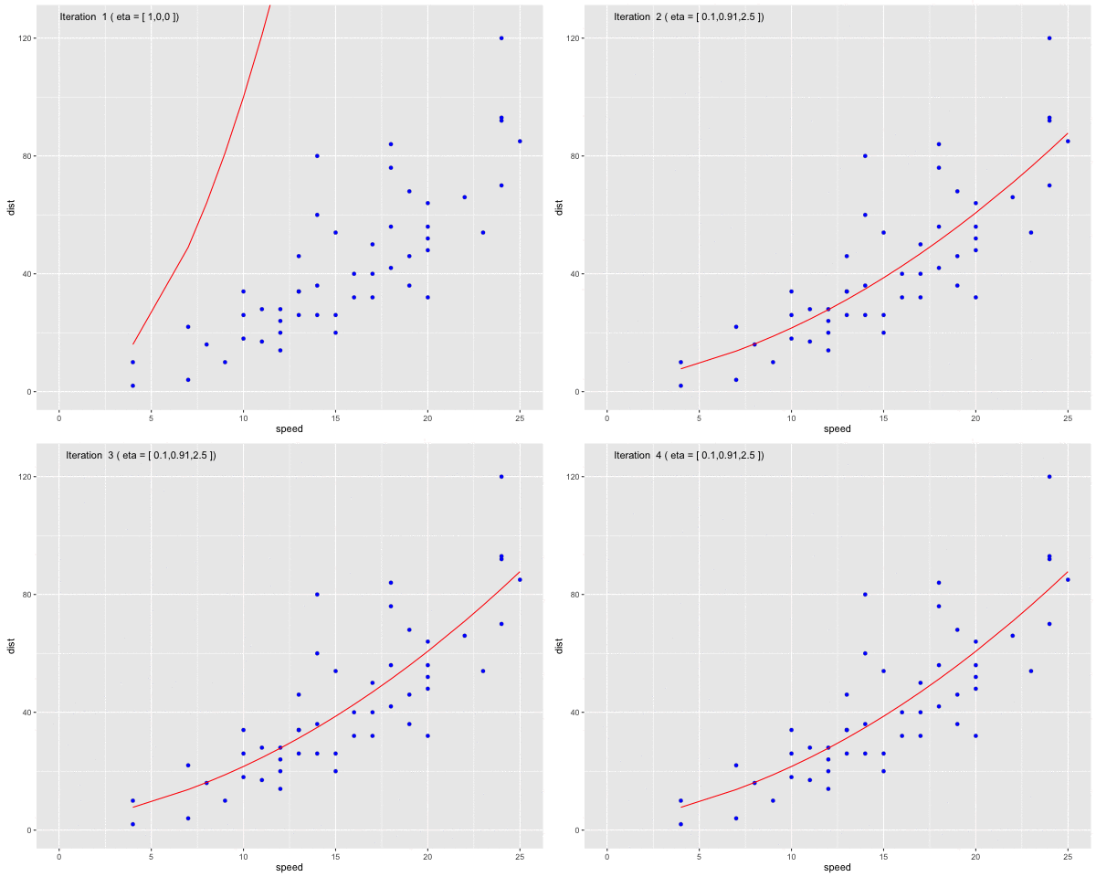
Fig 6. Use Gauss-Newton method to fit a curve line to the dataset