Table of Contents
Titanic is a entry level competition that Kaggle, a data science competition platform, has created to challenge novice data scientists so that they can have chance to earn some practical experiences before getting into advanced level competitions. I also spent hours on this challenge, and can’t wait any longer to share my experience.
1. Data munging
First thing first. We will spend sometimes on discovering the data. Data munging (also known as data wrangling) involves getting our hands dirty on the data to explore different aspects of the data, for example structure, statistics. I believe that there exists no standard guideline for data munging, except that we are encouraged to properly use all possible methods.
1.1 Data loading
We load the dataset first. In this case, I do not process the draw data but just a copy of it.
library(VIM) #aggr
library(ggplot2) #ggplot
################################################################################
# LOAD DATA
################################################################################
train_raw <- read.csv("data/train.csv", na.strings = c("NA", ""))

# Back up
train <- train_raw
Next, we discover the structure and data types of the data.
str(train, strict.width = "wrap")## 'data.frame': 891 obs. of 12 variables:
## $ PassengerId: int 1 2 3 4 5 6 7 8 9 10 ...
## $ Survived : int 0 1 1 1 0 0 0 0 1 1 ...
## $ Pclass : int 3 1 3 1 3 3 1 3 3 2 ...
## $ Name : Factor w/ 891 levels "Abbing, Mr. Anthony",..: 109 191 358 277 16
## 559 520 629 417 581 ...
## $ Sex : Factor w/ 2 levels "female","male": 2 1 1 1 2 2 2 2 1 1 ...
## $ Age : num 22 38 26 35 35 NA 54 2 27 14 ...
## $ SibSp : int 1 1 0 1 0 0 0 3 0 1 ...
## $ Parch : int 0 0 0 0 0 0 0 1 2 0 ...
## $ Ticket : Factor w/ 681 levels "110152","110413",..: 524 597 670 50 473
## 276 86 396 345 133 ...
## $ Fare : num 7.25 71.28 7.92 53.1 8.05 ...
## $ Cabin : Factor w/ 147 levels "A10","A14","A16",..: NA 82 NA 56 NA NA 130
## NA NA NA ...
## $ Embarked : Factor w/ 3 levels "C","Q","S": 3 1 3 3 3 2 3 3 3 1 ...Currently, Name, Ticket, Cabin are factors. We’ll convert them to characters.
## Convert Name, Ticket, Cabin to character
indx <- c("Name", "Ticket", "Cabin")
train[indx] <- lapply(train[indx], as.character)

str(train, strict.width = "wrap")
## 'data.frame': 891 obs. of 12 variables:
## $ PassengerId: int 1 2 3 4 5 6 7 8 9 10 ...
## $ Survived : int 0 1 1 1 0 0 0 0 1 1 ...
## $ Pclass : int 3 1 3 1 3 3 1 3 3 2 ...
## $ Name : chr "Braund, Mr. Owen Harris" "Cumings, Mrs. John Bradley
## (Florence Briggs Thayer)" "Heikkinen, Miss. Laina" "Futrelle, Mrs.
## Jacques Heath (Lily May Peel)" ...
## $ Sex : Factor w/ 2 levels "female","male": 2 1 1 1 2 2 2 2 1 1 ...
## $ Age : num 22 38 26 35 35 NA 54 2 27 14 ...
## $ SibSp : int 1 1 0 1 0 0 0 3 0 1 ...
## $ Parch : int 0 0 0 0 0 0 0 1 2 0 ...
## $ Ticket : chr "A/5 21171" "PC 17599" "STON/O2. 3101282" "113803" ...
## $ Fare : num 7.25 71.28 7.92 53.1 8.05 ...
## $ Cabin : chr NA "C85" NA "C123" ...
## $ Embarked : Factor w/ 3 levels "C","Q","S": 3 1 3 3 3 2 3 3 3 1 ...1.2 Missing data
We’ll visualise the missing data pattern of our data by using the function aggr of the package VIM.
# Missing data
missing_plot <- aggr(train, col=c('navyblue','red'), numbers=TRUE,
                  sortVars=TRUE, labels=names(train), cex.axis=.7, gap=3,
                  ylab=c("Histogram of missing data","Pattern"))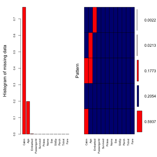
##
##  Variables sorted by number of missings:
##     Variable       Count
##        Cabin 0.771043771
##          Age 0.198653199
##     Embarked 0.002244669
##  PassengerId 0.000000000
##     Survived 0.000000000
##       Pclass 0.000000000
##         Name 0.000000000
##          Sex 0.000000000
##        SibSp 0.000000000
##        Parch 0.000000000
##       Ticket 0.000000000
##         Fare 0.000000000
Our visualisation tells us that there are 77% of missing data in Cabin, 20% in Age and exactly 0.2% in Embarked (which is exactly 2 missing records).
1.3. Data facets
# Find the relation between Survived, Pclass, Age, and Fare
ggplot(train, aes(x=Fare, y=Age)) +
  geom_point() +
  facet_grid(Survived ~ Pclass)
## Warning: Removed 177 rows containing missing values (geom_point).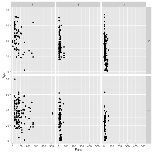
# Find the relation between Survived, Embarked, Age, and Fare
ggplot(train, aes(x=Fare, y=Age)) +
  geom_point() +
  facet_grid(Survived ~ Embarked)
## Warning: Removed 177 rows containing missing values (geom_point).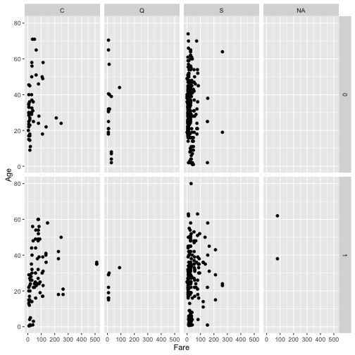
## Find the relation between Survived, Sibsp
ggplot(data = train, mapping = aes(x = SibSp)) +
  geom_histogram()
## `stat_bin()` using `bins = 30`. Pick better value with `binwidth`.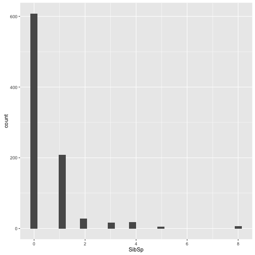
## Find the relation between Survived, Parch
ggplot(data = train, mapping = aes(x = Parch)) +
  geom_histogram()
## `stat_bin()` using `bins = 30`. Pick better value with `binwidth`.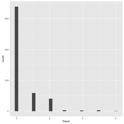
## Find the relation between Survived, Embarked
ct_table <- as.data.frame(table(train$Embarked, train$Survived))
names(ct_table) <- c("Embarked", "Survived", "Quantity")
ggplot(data = ct_table,
       mapping = aes(x = Survived, y = Quantity, fill = Embarked)) +
  geom_bar(stat = "identity")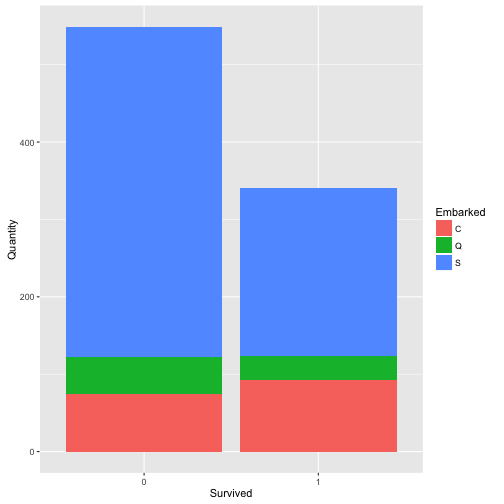
## Find the relation between Survived, Pclass
ct_table <- as.data.frame(table(train$Pclass, train$Survived))
names(ct_table) <- c("Pclass", "Survived","Quantity")
ggplot(data = ct_table,
       mapping = aes(x = Survived, y = Quantity, fill = Pclass)) +
  geom_bar(stat = "identity")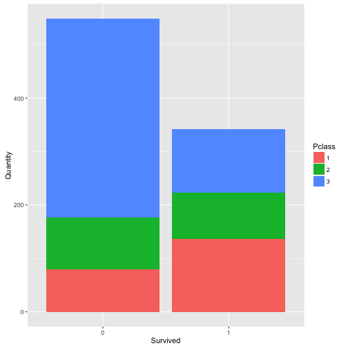
## Find the relation between Survived, Sex
ct_table <- as.data.frame(table(train$Sex, train$Survived))
names(ct_table) <- c("Sex", "Survived", "Quantity")
ggplot(data = ct_table,
       mapping = aes(x = Survived, y = Quantity, fill = Sex)) +
  geom_bar(stat = "identity") +
  ggtitle("Distribution of Survived by Sex") +
  xlab("Survived") +
  ylab("# of Passengers")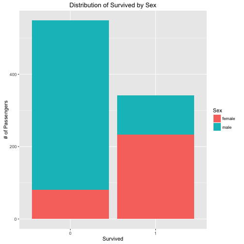
2. Modeling
################################################################################
# LOAD LIBRARY
################################################################################
library(mice) #missing
library(caret)
2.1. Feature Engineer
Next, we will extract first name, last name and title of passengers from Name, making 3 new columns in the dataset, which are FName, Title, LName.
#########################################
# LASTNAME & FIRSTNAME & TITLE
#########################################
name <- strsplit(train$Name, split='[,.]')

# First name
train$FName <- sapply(c(1:length(name)), function(x, name)
  return (trimws(name[[x]][1], which = "both")), name = name)

# Title
train$Title <- sapply(c(1:length(name)), function(x, name)
  return (trimws(name[[x]][2], which = "both")), name = name)

# Last name
lname <- sapply(c(1:length(name)), function(x, name)
  return (trimws(name[[x]][3], which = "both")), name = name)

lname_splt <- strsplit(lname, split ='[()]')

train$LName <- sapply(c(1:length(lname_splt)), function(x, lname_splt)
  return (trimws(lname_splt[[x]][1], which = "both")), lname_splt = lname_splt)

# Some don't have lastname, need to impute
lname_imp <- sapply(c(1:length(lname_splt)), function(x, lname_splt)
  return (trimws(lname_splt[[x]][2], which = "both")), lname_splt = lname_splt)
lname_missing_idx <- which(train$LName == "")
train$LName[lname_missing_idx] <- lname_imp[lname_missing_idx]

train$LName <- as.factor(train$LName)
summary(train$LName)
## William John James
## 11 10 9
## Mary Joseph Samuel
## 7 5 5
## Thomas Bertha Edward
## 5 4 4
## George Ivan Martin
## 4 4 4
## William Henry William John Alfred
## 4 4 3
## Alice Anna Anna Sofia
## 3 3 3
## Benjamin Elizabeth Emil
## 3 3 3
## Frederick Harry Johan
## 3 3 3
## Patrick Tannous Victor
## 3 3 3
## Albert Albert Adrian Alexander
## 2 2 2
## Alexander Oskar Anders Johan Antoni
## 2 2 2
## Arthur Charles Alexander Charles H
## 2 2 2
## Charles Henry David Dickinson H
## 2 2 2
## Edgar Joseph Edwy Arthur Ellen "Nellie"
## 2 2 2
## Elmer Zebley Ernest Courtenay Ernst Gilbert
## 2 2 2
## Frank John Frederick Charles Frederick Maxfield
## 2 2 2
## Frederick William George Henry Gerious
## 2 2 2
## Hanna Hanora "Nora" Harvey
## 2 2 2
## Henry Henry Birkhardt Henry Sleeper
## 2 2 2
## Henry William Jacques Heath Jakob Alfred
## 2 2 2
## Jean Baptiste John Borland John Henry
## 2 2 2
## Josef Juha Juho
## 2 2 2
## Karl Alfred Kate Katherine "Katie"
## 2 2 2
## Lalio Lawrence Lee
## 2 2 2
## Luka Marija Maurice
## 2 2 2
## Michael Nicholas Norman Campbell
## 2 2 2
## Pekka Pietari Percival Peter Henry
## 2 2 2
## Richard Richard Leonard Samuel L
## 2 2 2
## Sidney Samuel Sinai Thomas Henry
## 2 2 2
## Thomas Jr Thomas William Solomon Victor de Satode
## 2 2 2
## Wilhelm William Arthur William Baird
## 2 2 2
## William Ernest William James William John Robert
## 2 2 2
## William Thomas William Thompson Abraham
## 2 2 1
## (Other)
## 629Looks like we get something here. There are a lot of people having the same last name. It hints us that they are likely families.
train$Family <- train$SibSp + train$Parch + 1In fact, there are many families traveled, and we can easily identify the size of the family by combining both SibSp and Parch. Doing that, if a passenger has 0s on SibSp and Parch, we would have a family size of 0. That doesn’t make sense. Thus, we have to +1.
Next, we have to find a way to increase the correctness of Family. We can see that
- A lot of people have the same
Ticket. - A lot of people have the same
LName.
Thus, we will create a new column, FamilyID, and identify families in the dataset based on two assumptions. First, people who have the same Ticket should be a family, or a group of passengers. Second, people who have the same LName could belong to a family, but only if they have the same Pclass and Embarked. It does not make sense if people in the same family stay in different classess, and/or embark from different places.
train$FamilyId <- NA##############
# Grouping by similar tickets
###############
# There are a lot of similar tickets, So if passengers have the same ticket,
# they should be a family or a least travel together
train$Ticket <- as.factor(train$Ticket)
# Find tickets ID that used by > 1 passengers
ticket <- data.frame(table(train$Ticket))
similar_ticket <- ticket[ticket$Freq > 1, 1]
# Assign all ticket to FamilyID as suitable familyID
# then remove ones that not in similar ticket
train$FamilyId <- train$Ticket
# Find positions that do not be removed
ticket_idx <- sapply(similar_ticket, function(x) (return (which(train$FamilyId == x))))
ticket_idx <- unlist(ticket_idx)
# Set NA to position not in idx
train$FamilyId[-ticket_idx] <- NA##############
# Grouping by similar last name, pclass, embarked
###############
# Assign the same familyID to people who have the same lname by using
# the pattern lname_embark_pclass
lname <- data.frame(table(train$LName))
similar_lname <- lname[lname$Freq > 1, 1]
lname_idx <- sapply(similar_lname, function(x) (return (which(train$LName == x))))
lname_idx <- unlist(lname_idx)
diff <- setdiff(lname_idx, ticket_idx)
train$FamilyId <- as.character(train$FamilyId)
train$FamilyId[diff] <- sapply(train$LName[diff], function (x) return
(gsub("[[:space:]]", "", x)))
##############
# Update Family(size) by FamilyID
###############
# People who have family ID but FamilySize = 1
idx <- intersect(which(!is.na(train$FamilyId)), which(train$Family == 1))
freq <- data.frame(table(train$FamilyId[idx]))
names(freq) <- c("FamilyId", "Freq")
freq$FamilyId <- as.character(freq$FamilyId)
train$FamilyId[which(is.na(train$FamilyId))] <- ""
for (i in 1:nrow(freq)) {
train$Family[which(train$FamilyId == freq$FamilyId[i])] <- freq$Fre[i]
}After enhancing Family, we will have a look at our new feature Title. We can see that there are a variety of factors in Title. We reduce the number of factors by grouping them.
##############
# TITLE
###############
train$Title <- as.factor(train$Title)
summary(train$Title)
## Capt Col Don Dr Jonkheer
## 1 2 1 7 1
## Lady Major Master Miss Mlle
## 1 2 40 182 2
## Mme Mr Mrs Ms Rev
## 1 517 125 1 6
## Sir the Countess
## 1 1train$Title <- as.character(train$Title)
# Too many factors in Title, we need to merge them
train$Title[which(train$Title == "Capt")] <- "Mr"
train$Title[which(train$Title == "Col")] <- "Mr"
train$Title[which(train$Title == "Major")] <- "Mr"
train$Title[which(train$Title == "Don")] <- "Mr"
train$Title[which(train$Title == "Dr")] <- "Mr"
train$Title[which(train$Title == "Jonkheer")] <- "Mr"
train$Title[which(train$Title == "Rev")] <- "Mr"
train$Title[which(train$Title == "Sir")] <- "Mr"
train$Title[which(train$Title == "Mme")] <- "Mr"
train$Title[which(train$Title == "Lady")] <- "Mrs"
train$Title[which(train$Title == "the Countess")] <- "Mrs"
train$Title[which(train$Title == "Ms")] <- "Miss"
train$Title[which(train$Title == "Mlle")] <- "Miss"
train$Title <- as.factor(train$Title)
summary(train$Title)## Master Miss Mr Mrs
## 40 185 539 1272.2. Missing data imputation
# Fare == 0 doesnt make sense, thus should be missing values
train$Fare[which(train$Fare == 0)] <- NA
#########################################
# CABIN
#########################################
# More than 70% of Cabin is missing, thus we have to remove
train$Cabin <- NULL#########################################
# EMBARKED
#########################################
# Impute Embarked
train$Embarked[which(is.na(train$Embarked))] <- "S"We use multiple imputation by chained equation to impute missing values in Fare and Age. We will use Sex, Title, Fare, Pclass as predictors to impute. More importantly, because it does not make sense if imputed values of Fare and Age are negative, we have to squeeze values into two corresponding ranges, (1, 80) for Age and (1, 500) for Fare.
#########################################
# AGE
#########################################
# 19% of Age is missing. We'll find a way to impute the data
temp_train <- train[, c("Sex", "Age", "Title", "Fare", "Pclass")]
# Impute age
post <- mice(temp_train[, ], maxit = 0)$post
post["Age"] <- "imp[[j]][,i] <- squeeze(imp[[j]][,i], c(1,80))"
post["Fare"] <- "imp[[j]][,i] <- squeeze(imp[[j]][,i], c(1,500))"
restricted <- mice(temp_train, m = 5, post = post, seed = 567, method = 'norm')
##
## iter imp variable
## 1 1 Age Fare
## 1 2 Age Fare
## 1 3 Age Fare
## 1 4 Age Fare
## 1 5 Age Fare
## 2 1 Age Fare
## 2 2 Age Fare
## 2 3 Age Fare
## 2 4 Age Fare
## 2 5 Age Fare
## 3 1 Age Fare
## 3 2 Age Fare
## 3 3 Age Fare
## 3 4 Age Fare
## 3 5 Age Fare
## 4 1 Age Fare
## 4 2 Age Fare
## 4 3 Age Fare
## 4 4 Age Fare
## 4 5 Age Fare
## 5 1 Age Fare
## 5 2 Age Fare
## 5 3 Age Fare
## 5 4 Age Fare
## 5 5 Age Faretrain_temp <- complete(restricted, 1)
train$Age <- train_temp$Age
train$Fare <- train_temp$FareThe next move is to ensure there is no missing values in the data.
# Assure that no more missing
missing_plot <- aggr(train, col=c('navyblue','red'), numbers=TRUE,
                     sortVars=TRUE, labels=names(train), cex.axis=.7, gap=3,
                     ylab=c("Histogram of missing data","Pattern"))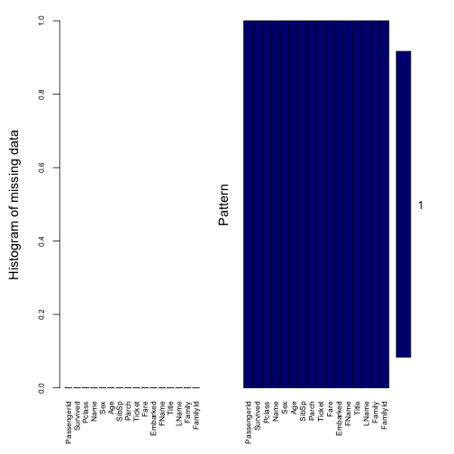
##
##  Variables sorted by number of missings:
##     Variable Count
##  PassengerId     0
##     Survived     0
##       Pclass     0
##         Name     0
##          Sex     0
##          Age     0
##        SibSp     0
##        Parch     0
##       Ticket     0
##         Fare     0
##     Embarked     0
##        FName     0
##        Title     0
##        LName     0
##       Family     0
##     FamilyId     0
2.3. Categorizing data
################################################################################
# CATEGORISE DATA & CREATE DUMMY VARIABLES FOR NOMINAL DATA
################################################################################
# Pclass
for(level in unique(train$Pclass)){
  train[paste("Pclass", level, sep = "_")] <- ifelse(train$Pclass == level, 1, 0)
}

# Embarked
for(level in unique(train$Embarked)){
  train[paste("Embarked", level, sep = "_")] <- ifelse(train$Embarked == level, 1, 0)
}

# Sibsp
train$SibSp <- as.factor(findInterval(train$SibSp, c(1, 2)))

for(level in unique(train$SibSp)){
  train[paste("SibSp", level, sep = "_")] <- ifelse(train$SibSp == level, 1, 0)
}

# Parch
train$Parch <- as.factor(findInterval(train$Parch, c(1, 3)))

for(level in unique(train$Parch)){
  train[paste("Parch", level, sep = "_")] <- ifelse(train$Parch == level, 1, 0)
}

# Sex
for(level in unique(train$Sex)){
  train[paste("Sex", level, sep = "_")] <- ifelse(train$Sex == level, 1, 0)
}

# Fare
train$Fare_factor <- as.factor(findInterval(train$Fare, c(32)))

for(level in unique(train$Fare_factor)){
  train[paste("Fare_factor", level, sep = "_")] <- ifelse(train$Fare_factor == level, 1, 0)
}

# Age
train$Age_factor <- as.factor(findInterval(train$Age, c(21.1, 37, 60)))

for(level in unique(train$Age_factor)){
  train[paste("Age_factor", level, sep = "_")] <- ifelse(train$Age_factor == level, 1, 0)
}

# FamilySize
train$FamilySize <- as.factor(findInterval(train$Family, c(2, 5)))
for(level in unique(train$Age_factor)){
  train[paste("FamilySize", level, sep = "_")] <- ifelse(train$Age_factor == level, 1, 0)
}
2.4. Model construction
################################################################################
# BUIDING MODEL
################################################################################
set.seed(234)

# Split data
inTraining <- createDataPartition(train$Survived, p = .5, list = FALSE)
training <- train[inTraining,]
testing  <- train[-inTraining,]

# Train control
fitControl <- trainControl(## 10-fold CV
  method = "repeatedcv",
  number = 10,
  repeats = 10,
  allowParallel = TRUE)

# Model tuning
grid <-  expand.grid(mtry = seq(1, 7, 1))

# Model
model <- train(as.factor(Survived) ~ Sex_male +
                 Pclass_3 + Pclass_1 + Embarked +
                 Age +
                 Fare + FamilySize,
               data = training,
               method = "parRF",
               trControl = fitControl,
               verbose = TRUE,
               tuneGrid = grid,
               preProc = c("center", "scale"),
               metric = "Kappa")
## Loading required package: e1071## Loading required package: randomForest## randomForest 4.6-12## Type rfNews() to see new features/changes/bug fixes.##
## Attaching package: 'randomForest'## The following object is masked from 'package:ggplot2':
##
## margin## Loading required package: foreach## Warning: executing %dopar% sequentially: no parallel backend registeredmodel## Parallel Random Forest
##
## 446 samples
## 7 predictor
## 2 classes: '0', '1'
##
## Pre-processing: centered (9), scaled (9)
## Resampling: Cross-Validated (10 fold, repeated 10 times)
## Summary of sample sizes: 402, 402, 401, 401, 401, 401, ...
## Resampling results across tuning parameters:
##
## mtry Accuracy Kappa
## 1 0.7898411 0.5352829
## 2 0.8122511 0.5898479
## 3 0.8086648 0.5865441
## 4 0.8106499 0.5935032
## 5 0.8073165 0.5889437
## 6 0.8058973 0.5865967
## 7 0.7993973 0.5751578
##
## Kappa was used to select the optimal model using the largest value.
## The final value used for the model was mtry = 4.# Plot model performance
plot(model)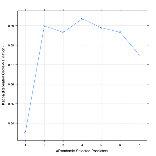
# Check feature importances
varImp(model)
## parRF variable importance
##
## Overall
## Sex_male 100.000
## Age 83.674
## Fare 73.573
## Pclass_3 25.171
## FamilySize2 9.530
## FamilySize1 8.053
## Pclass_1 7.275
## EmbarkedS 6.543
## EmbarkedQ 0.000# Testing
pred <- predict(model, newdata = testing)
error <- mean(pred != testing$Survived)
print(paste("Accuracy ", 1 - error))## [1] "Accuracy 0.835955056179775"3. Testing
We will re-apply all our necessary step above to the test data given by Kaggle. This model is able to achieve 0.8038. The full source code can be found in Github.