This is a research experiment of using mice package (Buuren and Groothuis-Oudshoorn, 2011) to impute missing values in multivariate data. Basically, mice uses Fully Conditional Specification (FCS) method, whereas chained equation is considered an alias of that term. According to Liu and De (2015), FCS is more relaxed than the conventional method Joint Modeling (JM) in terms of specifiying distribution of the missing data.
In this experiment, we will use an open source dataset Titanic (Kaggle, 2012) as the sample data of the experiment.
1. Multiple imputation vs Single imputation
Both multiple and single imputation techniques are ones that can be used to replace missing values in the data by plausible values. In single imputation, we substitute the missing values of the data by a single value. For example, we can replace missing values of a variable by the most common value, or the mean/median value (in case that variable is continuous). Multiple imputation is different in a sense that missing values are replaced by multiple plausible values. Using mice package, we can even have multiple version of imputed data by trying to impute the data more than one time.
2. Notation
- $\mathbf{Y_j}$ $(j = 1,…, p)$: one of $p$ incomplete variables.
- The observed and missing parts of $Y_j$ are denoted by $\mathbf{Y_j^{obs}}$ and $\mathbf{Y_j^{mis}}$.
- $Y^{obs} = (Y^{obs},…,Y^{obs}_p)$: observed data in Y.
- $Y^{mis} = (Y^{mis},…,Y^{mis}_p)$: missing data in Y.
- $\mathbf{m \ge 1}$: the number of imputation.
- $\mathbf{Q}$: predicted model that would be trained on $Y$.
3. Features
mice introduces a modular approach to impute data. The imputation framework offered by mice comprises of 3 steps: imputation, analysis and pooling (Figure 1).
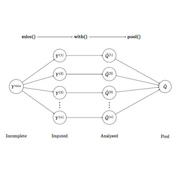
mice()Impute incomplete data, creating imputed versions of the data $Y^{(1)}$, $Y^{(2)}$, …, $Y^{(m)}$.with()Estimate the predicted model $Q$ on each imputed dataset $Y^{(i)}$, creating multiple versions of the model, which are $\hat{Q}^{(1)}$, $\hat{Q}^{(2)}$,…, $\hat{Q}^{(m)}$pool()Pool $\hat{Q}^{(1)}$, $\hat{Q}^{(2)}$,…, $\hat{Q}^{(m)}$ into one estimates $\bar{Q}$
A notable feature of this imputation model is that we use our predicted model of interest $Q$ to analyse the imputed data by ourself. By doing that, we can specifically select the best imputed data that suits our investigation.
4. Experiment
4.1. Missing value inspection
First and foremost, load the package and data. In this experiment, we will use Titanic data free available from Kaggle.
# Load library
library(mice) # Imputation
library(VIM) #aggr, marginplot
library(lattice) #stripplot
# Load data
dt <- read.csv("data/titanic.csv", na.strings = c("NA", ""))
# Inspect the data structure
str(dt, strict.width = "wrap")
## 'data.frame': 891 obs. of 12 variables:
## $ PassengerId: int 1 2 3 4 5 6 7 8 9 10 ...
## $ Survived : int 0 1 1 1 0 0 0 0 1 1 ...
## $ Pclass : int 3 1 3 1 3 3 1 3 3 2 ...
## $ Name : Factor w/ 891 levels "Abbing, Mr. Anthony",..: 109 191 358 277 16
## 559 520 629 417 581 ...
## $ Sex : Factor w/ 2 levels "female","male": 2 1 1 1 2 2 2 2 1 1 ...
## $ Age : num 22 38 26 35 35 NA 54 2 27 14 ...
## $ SibSp : int 1 1 0 1 0 0 0 3 0 1 ...
## $ Parch : int 0 0 0 0 0 0 0 1 2 0 ...
## $ Ticket : Factor w/ 681 levels "110152","110413",..: 524 597 670 50 473
## 276 86 396 345 133 ...
## $ Fare : num 7.25 71.28 7.92 53.1 8.05 ...
## $ Cabin : Factor w/ 147 levels "A10","A14","A16",..: NA 82 NA 56 NA NA 130
## NA NA NA ...
## $ Embarked : Factor w/ 3 levels "C","Q","S": 3 1 3 3 3 2 3 3 3 1 ...# Remove unnecessary columns
dt[, c("PassengerId", "Name", "Cabin", "Ticket")] <- NULL
# Summary the data
summary(dt) ## Survived Pclass Sex Age
## Min. :0.0000 Min. :1.000 female:314 Min. : 0.42
## 1st Qu.:0.0000 1st Qu.:2.000 male :577 1st Qu.:20.12
## Median :0.0000 Median :3.000 Median :28.00
## Mean :0.3838 Mean :2.309 Mean :29.70
## 3rd Qu.:1.0000 3rd Qu.:3.000 3rd Qu.:38.00
## Max. :1.0000 Max. :3.000 Max. :80.00
## NA's :177
## SibSp Parch Fare Embarked
## Min. :0.000 Min. :0.0000 Min. : 0.00 C :168
## 1st Qu.:0.000 1st Qu.:0.0000 1st Qu.: 7.91 Q : 77
## Median :0.000 Median :0.0000 Median : 14.45 S :644
## Mean :0.523 Mean :0.3816 Mean : 32.20 NA's: 2
## 3rd Qu.:1.000 3rd Qu.:0.0000 3rd Qu.: 31.00
## Max. :8.000 Max. :6.0000 Max. :512.33
## # Fare = 0 doesn't make sense, set 0 values in Fare as missing values
dt$Fare[dt$Fare == 0] <- NAOur data contains a lot of missing values. We will use different methods to inspect them. First, we will use md.pattern method to inspect missing-data patterns.
md.pattern(dt)## Survived Pclass Sex SibSp Parch Embarked Fare Age
## 705 1 1 1 1 1 1 1 1 0
## 169 1 1 1 1 1 1 1 0 1
## 7 1 1 1 1 1 1 0 1 1
## 2 1 1 1 1 1 0 1 1 1
## 8 1 1 1 1 1 1 0 0 2
## 0 0 0 0 0 2 15 177 194Let’s intepret information from the retrieved table. Note that in the table, 0 represents missing in the data. Look at the table by row, the table tells us that we have 705 complete rows, 169 rows where only Age is missing, 7 rows where only Fare is missing, 2 rows where Embarked is missing, and 8 rows where both Fare and Age are missing. Vertically, the tables tells us that Embarked has 2 missing values, Fare 15, and Age 177. In overall, we have 194 missing values in the data, and 169 + 7 + 2 + 8 = 186 incomplete rows.
Besides md.pattern, we can visually inspect missing patterns of the data using the package VIM. First, we will use aggr to aggregate missing values.
aggr(dt, col = c("navyblue","red"), sortVars = TRUE, numbers = TRUE)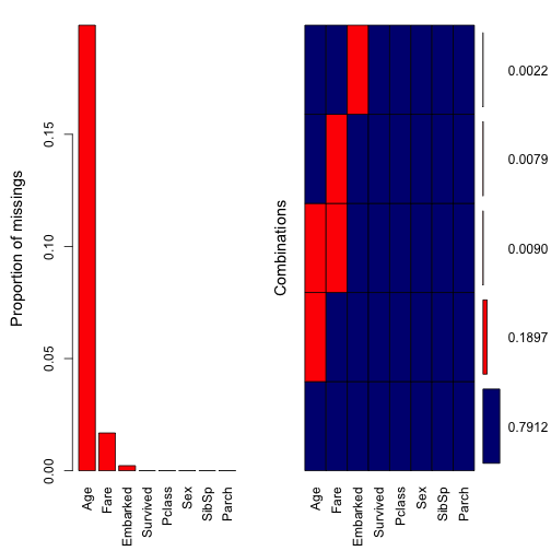
##
##  Variables sorted by number of missings:
##  Variable       Count
##       Age 0.198653199
##      Fare 0.016835017
##  Embarked 0.002244669
##  Survived 0.000000000
##    Pclass 0.000000000
##       Sex 0.000000000
##     SibSp 0.000000000
##     Parch 0.000000000
The method aggr is essentially similar to md.patterns, except that aggr displays missing values in portion. For example, roughly 20% (177 rows) of Age are incomplete, 1.6% (15 rows) of Fare missing, and 0.2% (2 rows) of Embarked missing. There are roughly 0.9% (8 rows) of the data where both Age and Fare are missing. Thus, it seems more convenient when combine both md.pattern and aggr together to inspect missing values of the data.
We can also observe missing values by pair. The function marginplot is perfect for this purpose. We will use marginplot to inspect missing patterns of the pair Age and Fare.
marginplot(dt[, c("Fare", "Age")], col = c("navyblue", "red"),
           numbers = TRUE, pch = 19)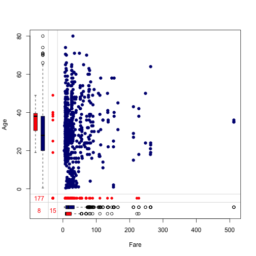
Let’s intepret information given by the plot.
- Blue points in the main area indicates the number of rows that both
AgeandFareare complete. The red points in the left side indicates missing values ofFarewhenAgeis observed. Similarly, the red points in the bottom margin indicates missing values ofAgewhenFareis observed. - Three numbers tells us that there are 15 missing values in
FarewhenAgeis observed, 177 missing values inAgewhenFareis observed, and 8 commonly missing values for both. - The blue and red boxplots summarise the marginal distribution of complete and incomplete rows. For example, the distribution of complete
Agevalues is (0, 80) years old, the distribution of missing value inFarewhenAgeis observed is from (20, 50) years old (i.e., 15 passengers who has missing values ofFareare from 20 to 50 years old).
4.2. Data imputation with mice()
We can simply impute the data by using the function mice(). For example,
# Impute missing values
imp <- mice(dt, maxit = 20)
By default, mice() will create 5 version of imputed data (i.e., m = 5), and for each version, the default number of iterations is also 5 (i.e., maxit = 5). According to the authors, the convergence of Gibbs sampling often happens when maxit is between 10 and 20.
# Extract the 1st version of the imputed data using complete()
dt_imp_1 <- complete(imp, 1)
summary(dt_imp_1)
## Survived Pclass Sex Age
## Min. :0.0000 Min. :1.000 female:314 Min. : 0.42
## 1st Qu.:0.0000 1st Qu.:2.000 male :577 1st Qu.:20.00
## Median :0.0000 Median :3.000 Median :28.00
## Mean :0.3838 Mean :2.309 Mean :28.83
## 3rd Qu.:1.0000 3rd Qu.:3.000 3rd Qu.:37.00
## Max. :1.0000 Max. :3.000 Max. :80.00
## SibSp Parch Fare Embarked
## Min. :0.000 Min. :0.0000 Min. : 4.013 C:170
## 1st Qu.:0.000 1st Qu.:0.0000 1st Qu.: 7.925 Q: 77
## Median :0.000 Median :0.0000 Median : 14.500 S:644
## Mean :0.523 Mean :0.3816 Mean : 32.518
## 3rd Qu.:1.000 3rd Qu.:0.0000 3rd Qu.: 31.275
## Max. :8.000 Max. :6.0000 Max. :512.329We can see that missing values no longer exist in the data. Let’s see how the data is imputed across 5 versions. First begin with Embarked
# Embarked
idx <- which(is.na(dt$Embarked)) # get index of missing values in the original data
sapply(c(1:5), function(x) {(complete(imp, x)$Embarked[idx])})
## [,1] [,2] [,3] [,4] [,5]
## [1,] "C" "C" "C" "S" "C"
## [2,] "C" "S" "S" "S" "C"So, mice() imputed missing values in Embarked with different values. Note that in the original data, there are 644 rows of S. So I suspect the imputed values are likely (S,S).
Next, we will explore the distribution of imputed values of Age and Fare. It can be seen from both plots that the distribution of imputed values are similar to that of observed values.
# Age
dt_imp_1 <- complete(imp, "long", inc = TRUE)
col <- rep(c("blue", "red")[1+as.numeric(is.na(imp$data$Age))], 6)
stripplot(Age~.imp, data = dt_imp_1, jit = TRUE, fac = 0.8, col = col,
          xlab = "Imputation Number")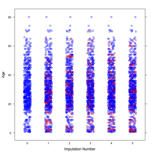
# Fare
col <- rep(c("blue", "red")[1+as.numeric(is.na(imp$data$Fare))], 6)
stripplot(Fare~.imp, data = dt_imp_1, jit = TRUE, fac = 0.8, col = col,
          xlab = "Imputation Number")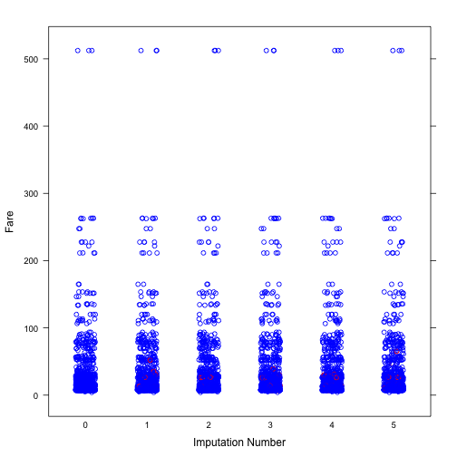
4.2. Data analysis with with()
After imputation, we will analyse imputed data using with(). As said, we analyse the imputed data by our predict model of interest $Q$.
fit <- with(imp, glm(Survived ~ Sex + Age + Fare + Pclass + SibSp + Parch
                     + Embarked, family = "binomial"))
4.3. Result pooling with pool()
pool(fit)## Call: pool(object = fit)
##
## Pooled coefficients:
## (Intercept) Sex2 Age Fare Pclass
## 5.721573191 -2.742309073 -0.044220471 0.001294004 -1.229816797
## SibSp Parch Embarked2 Embarked3
## -0.384499645 -0.080942900 0.008981836 -0.388565364
##
## Fraction of information about the coefficients missing due to nonresponse:
## (Intercept) Sex2 Age Fare Pclass SibSp
## 0.21052610 0.02914752 0.39931480 0.01121808 0.11571302 0.05188839
## Parch Embarked2 Embarked3
## 0.01208783 0.08927502 0.01918828summary(pool(fit))## est se t df Pr(>|t|)
## (Intercept) 5.721573191 0.649360179 8.81109340 92.70510 6.838974e-14
## Sex2 -2.742309073 0.206085341 -13.30666732 744.34461 0.000000e+00
## Age -0.044220471 0.009322114 -4.74360962 29.31085 5.051145e-05
## Fare 0.001294004 0.002370095 0.54597163 857.30898 5.852275e-01
## Pclass -1.229816797 0.160296256 -7.67214923 237.70923 4.343192e-13
## SibSp -0.384499645 0.112323317 -3.42315072 560.94776 6.641687e-04
## Parch -0.080942900 0.120734754 -0.67041923 853.63150 5.027719e-01
## Embarked2 0.008981836 0.406651902 0.02208728 333.63553 9.823915e-01
## Embarked3 -0.388565364 0.240072851 -1.61853105 815.52976 1.059348e-01
## lo 95 hi 95 nmis fmi lambda
## (Intercept) 4.432018506 7.011127875 NA 0.21052610 0.193675922
## Sex2 -3.146886777 -2.337731369 NA 0.02914752 0.026542410
## Age -0.063277556 -0.025163385 177 0.39931480 0.359679804
## Fare -0.003357863 0.005945872 15 0.01121808 0.008914053
## Pclass -1.545599435 -0.914034160 0 0.11571302 0.108304116
## SibSp -0.605125331 -0.163873959 0 0.05188839 0.048514010
## Parch -0.317914664 0.156028863 0 0.01208783 0.009775928
## Embarked2 -0.790943030 0.808906703 NA 0.08927502 0.083831931
## Embarked3 -0.859798868 0.082668139 NA 0.01918828 0.0167858945. Convergence assessment
Convergence assessment of Gibbs sampling algorithm is important to check that if the algorithm is converged. According to the paper: “There is no clear-cut method for determining whether the Gibbs sampling algorithm has converged. What is often done is to plot one or more parameters against the iteration number” and “on convergence, the different streams should be freely intermingled with each other, without showing any definite trends. Convergence is diagnosed when the variance between different sequences is no larger than the variance with each individual sequence”.
plot(imp)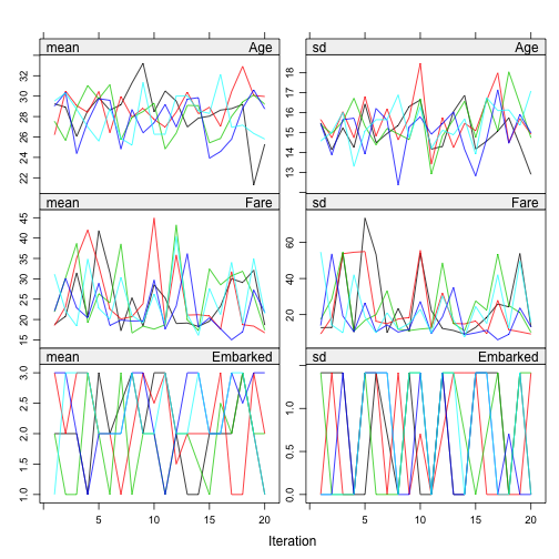
6. Conclusion
In this experiment, we have demonstrated how missing values in the data can be imputed using FCS technique. When compare FCS with JM technique, MICE is considered as a more adaptable method when we can select appropriate imputation models for variables on a case by case basis. For example, we can choose linear regression or Bayesian linear regression for continuous variables, and logistic regression or linear discriminant analysis for nominal variables.
mice package in R is a powerful and convenient library that enables multivariate imputation in a modular approach consisting of three subsequent steps. First, we can impute missing values by using a single mice() function, then effectively analyse imputed versions of data by using with() method with our own model of choice, and finally report the imputation result by using pool() method.
After this experiment, we believe that mice package is capable of supporting our future research experiments, where we would have chance to explore additional features of it, such as, implementing our own imputation models.
References
Buuren, S. & Groothuis-Oudshoorn, K. (2011, December). MICE: Mulitivariate Imputation by Chained Equations in R. Journal of Statistical Software, 45(3), 1–67. Retrieved from http://doc.utwente.nl/78938/
Kaggle. (2012, September). Titanic: machine learning from disaster. Retrieved from https://www.kaggle.com/c/titanic
Liu, Y. & De, A. (2015, July). Multiple Imputation by Fully Conditional Specification for Dealing with Missing Data in a Large Epidemiologic Study. International Journal of Statistics in Medical Research, 4(3), 287–295. doi:10.6000/1929-6029.2015.04.03.7