Table of Contents
I. From simple threshold neurons to perceptrons
1. Introduction
Perceptron is the earliest generation of artificial neural networks studied by Rosenblatt in 1958 (Rosenblatt, 1958). It is a progression of McCulloch-Pitts’s threshold neurons (McCulloch & Pitts, 1943), in which Rosenblatt basically made threshold neurons be able to learn by employing Hebbian learning (Hebb, 1949). In the book “Perceptrons” (Minsky & Papert, 1969), Minsky and Papert highlighted some strengths of perceptrons as well as identified their restrictions. A notable example of perceptrons’ limitations was demonstrated using XOR problem, in which perceptrons are incapable of learning to classify data points produced by the XOR function. The demonstrated limitations were thought applicable to not only perceptrons but also another kinds of neural networks. However, subsequent inventions in neural networks proved that it is not true.
2. Threshold neurons
In 1940, McCulloch-Pitts developed threshold neurons as an attempt to technically mimic biological neurons. A threshold neuron is characterised by the threshold function, by which inputs are mapped to outputs of either 0 or 1. More importantly, threshold neurons have no learning mechanism, because they have a fixed set of weights.
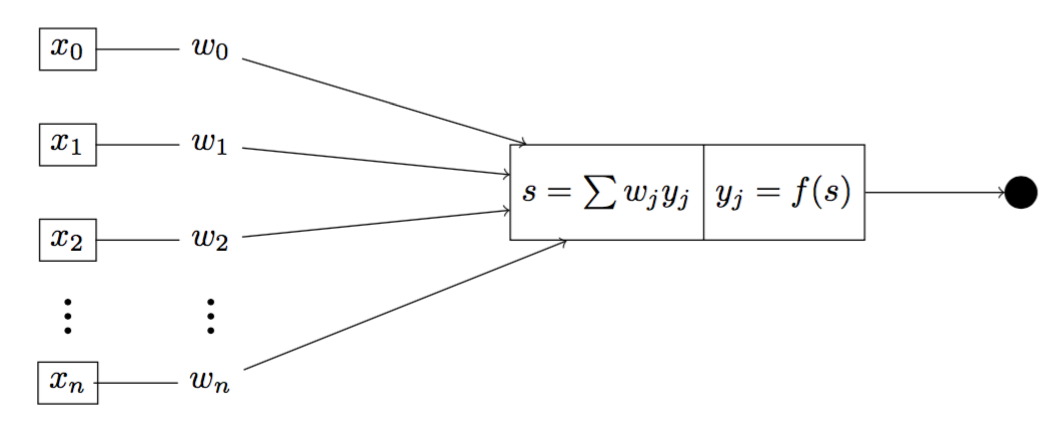
Fig 1. Illustration of a threshold neuron
Figure 1 is an illustration of a threshold neuron whose outputs are either 0 or 1. Inside the neuron, we have two distinct functions $\Sigma$ and $f(\cdot)$, by which we first calculate the sum of weighted inputs $s$ using $\Sigma$, and second the output using the threshold function $f(\cdot)$. We can calculate the output $y$ of the neuron by
\[y = f(s) = f(\sum_{j=1}^{N} w_jx_j) = f(\mathbf{w^Tx})\]where $f(\cdot)$ is given by
\[f(\cdot) = \begin{cases} \hfill 1 \hfill & \text{when $s \ge r$, where $r$ is any real number} \\ \hfill 0 \hfill & \text{otherwise} \\ \end{cases}\]3. Perceptron
In contrast to threshold neurons, perceptrons are able to adjust their weights during learning. At the beginning, we initialise the weight vector $\mathbf{w}$ by a random weight value ${w^{(0)}}$, and the learning rate $\eta$ by any random value $r$ satisfying $0 \le r \le 1$. We then start to go through every single observation ${x_j}$ of the input vector $\mathbf{x}$ and update $\mathbf{w}$ by the following rule.
- Compute the net input $u$ corresponding to $x_j$ such that $u = w^Tx_j$.
- Compute the output $\hat{y}_j$ given the threshold function $ f(u) = \begin{cases} 0 & \text{if } u < 0 \ 1 & \text{if } u \ge 0 \end{cases}$
- Compute the error $E$ such that $E = y_j - \hat{y}_j$.
- Update the weight $w^{(j+1)}$ by $w^{(j+1)} = w^{(j)} + \eta \, E \, x_j$.
- Repeat steps 1, 2, 3, 4 until $j = N$.
The updating rule of $\mathbf{w}$ can be understood that we only update $\mathbf{w}$ if and only if the predicted output $\hat{y}_j$ is different with the actual output $y_j$. If $E = 1$, we have $w^{(j+1)} = w^{(j)} + \eta \, x_j$. On the other hand, if $E = -1$, we have $w^{(j+1)} = w^{(j)} - \eta \, x_j$. We can summary three possibilities by
\[w^{(j+1)} = \begin{cases} w^{(j)} & \text{if $E = 0$, $y_j = \hat{y}_j$} \\ w^{(j)} - \eta \, x_j & \text{if $E = -1$, $y_j = 0$, $\hat{y}_j = 1$} \\ w^{(j)} + \eta \, x_j & \text{if $E = 1$, $y_j = 1$, $\hat{y}_j = 0$} \end{cases}\]4. Geometric interpretation
The learning algorithm of perceptrons can be understood geometrically. Suppose we have a plane defined by the weight vector $\mathbf{w} \in \mathbb{R}^2$ such that $w_0 + w_1 x_1 + w_2 x_2 = 0$ or $\mathbf{w^Tx} = 0$ where $x_0 = 1$. Since $\mathbf{w^Tx} = 0$, $\mathbf{w}$ is orthogonal to the plane (Figure 2).
More importantly, the plane $w^Tx = 0$ divides the space into two distinct half-planes, such that given any vector $\mathbf{u}$, we have $\mathbf{u \cdot w} \ge 0$ if $\mathbf{w}$ and $\mathbf{u}$ are on the same half-plane, otherwise $\mathbf{u \cdot w} < 0$. This can be proven by using the formula $\mathbf{u \cdot w} = \lVert u \rVert \cdot \lVert w \rVert \cdot cos \theta$, where $\theta$ is the angle between two vectors. Since $\lVert u \rVert \ge 0$, $\lVert w \rVert \ge 0$, we can conclude that $\mathbf{u \cdot w} \ge 0 $ if $0^{\circ} \le \theta \le 90^{\circ}$. Other other hand, $\mathbf{u \cdot w} < 0 $ if $\theta \ge 90^{\circ}$.
Based on that, we are now going to interpret the perceptron learning algorithm. When $E = -1$, (i.e., $y_j = 0$, $\hat{y}_j = 1$), two vectors \(\mathbf{u}\) and \(\mathbf{w}\) should be on different half-planes, but they are not. Thus, the plane needs to be rotated further away on the opposite direction of the vector $\mathbf{u}$ to increase the value of $\theta$. In contrast, when $E = 1$, (i.e., $y_j = 1$, $\hat{y}_j = 0$), $\mathbf{u}$ and $\mathbf{w}$ should be on the same half-plane, but they are not. Thus, the plane need to be rotated closer on the direction of the vector $\mathbf{u}$, making the value of $\theta$ decrease.
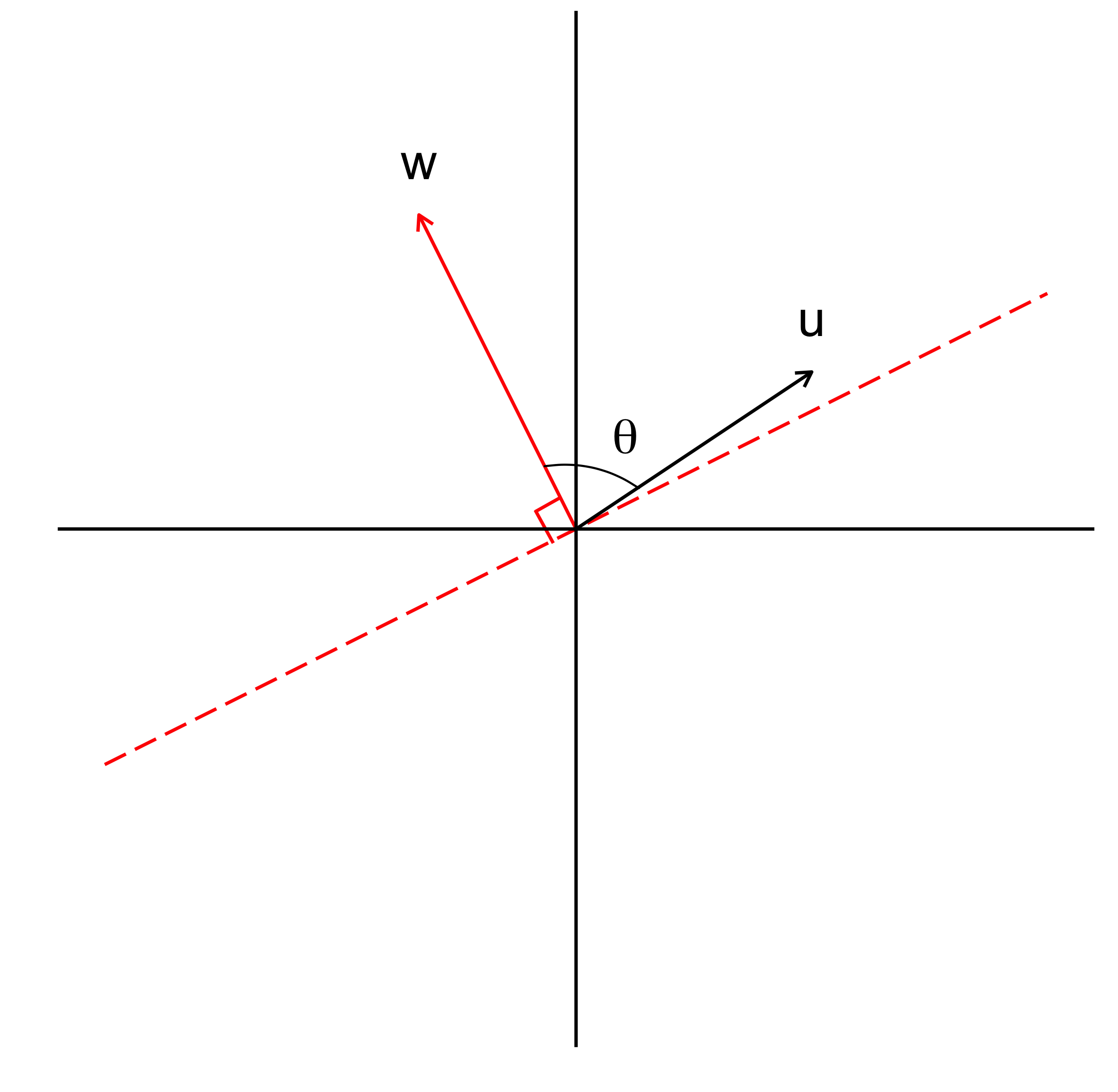
Fig 2. Visualisation of two-half planes divided by the plane $\mathbf{w^Tx = 0}$
Example A visualised example is provided to illustrate the operation of the perceptron learning algorithm. Given a set of data points in the table below, the perceptron learning function will be used to classify them.
At the beginning, we set the initial value of $\mathbf{w}$ equal to a random value and the learning rate $\eta$ equal to 1 (Figure 3a).
- We begin with $x_1$. Because $E = -1$, the plane rotates on the direction of $x_1$, updating $w_1 = w_0 - x_1$ (Figure 3b).
- At $x_2$, we have $E = 0$, the weight remains the same, thus $w_2 = w_1$ (Figure 3c).
- At $x_3$, we have $E = 1$, the plane needs to rotate on the direction of $x_3$, thus $w_3 = w_2 + x_3$ (Figure 3d)
Because the perceptron algorithm is unable to classify the data in 1 iteration. We need to repeat the process one more time. Figure 4 visualises how the perceptron learns in the 2nd iteration. At the end of the 2nd iteration, the perceptron converges when all data points are successfully classified.
| $x_1$ | $x_2$ | y |
|---|---|---|
| 1.5 | 1 | 0 |
| -1 | 1 | 1 |
| 0.5 | 0.5 | 1 |
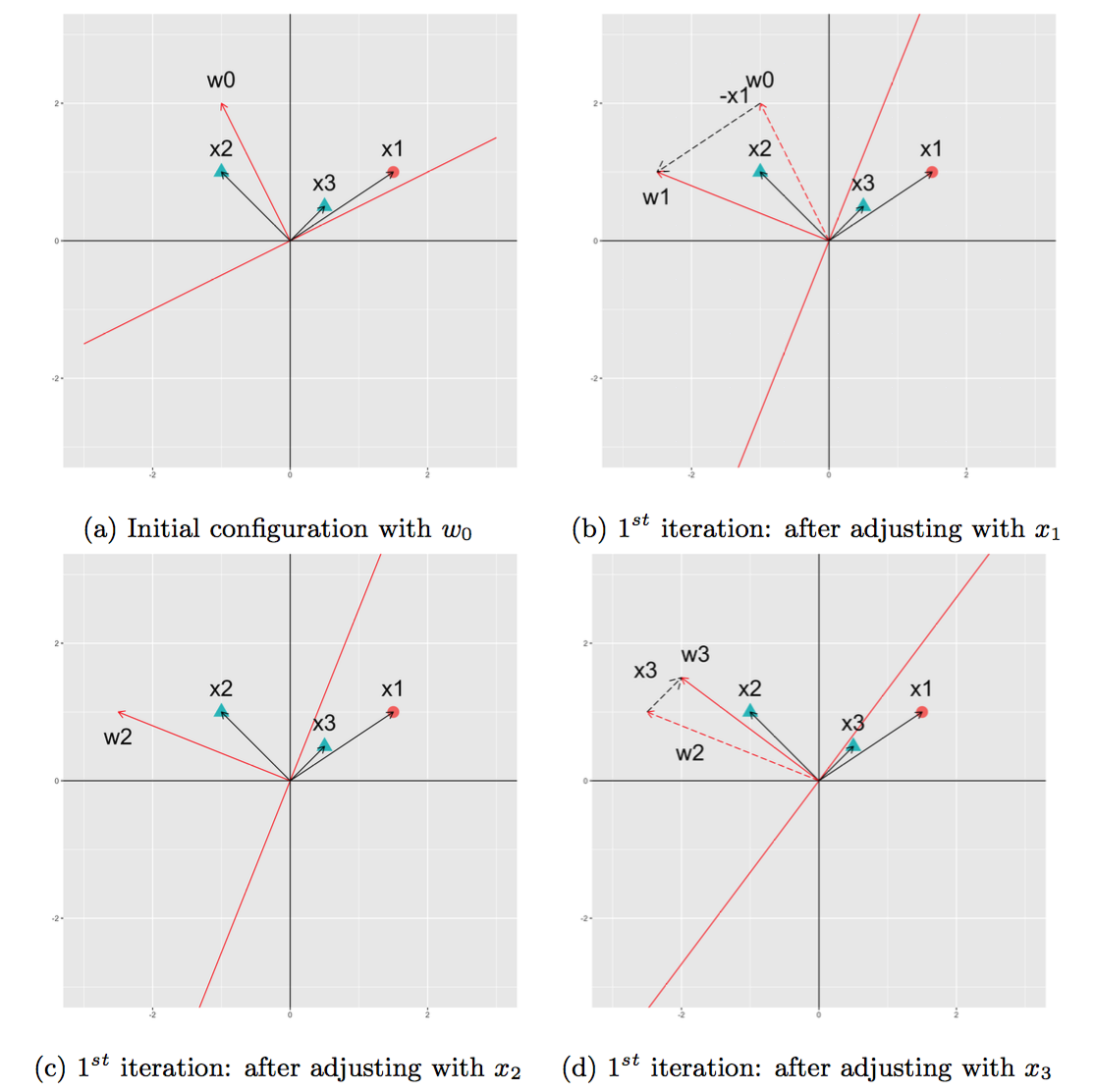
Fig 3. Changes of $\mathbf{w}$ in the 1st iteration
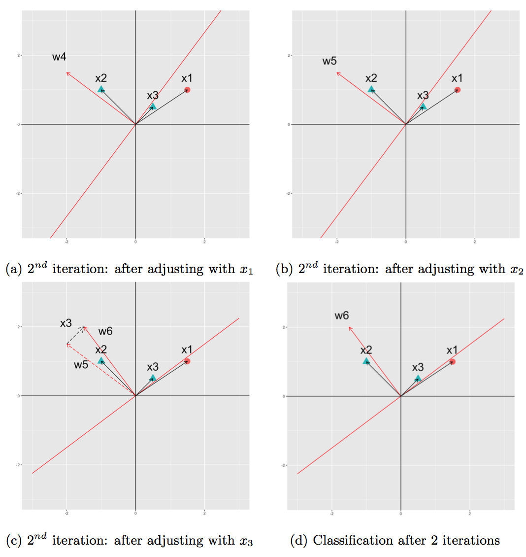
Fig 4. Changes of $\mathbf{w}$ in the 2nd iteration
5. Experiment
In this experiment, we are going to use perceptrons to classify the salmon data (Johnson & Wichern, 2007). This experiment is conducted using R. The visualised output of the plane created by the perceptron learning function is given in Figure 5 and 6.
Fig 5. Formation of the decision boundary step by step
We also conducted an additional experiment to verify an assumption that if the performance of the perceptron is higher when we increase the number of iterations. Figure 7 depicts the accuracy of the perceptron after numbers of epoch, given that an epoch indicates one pass of all training data points. According to the figure, we can see that the performance of the our model slightly improves from 0 epochs to 30 epochs, but after 30 epochs, it drops hugely. Thus, we can conclude that the performance of the model is not pertaining to the number of epochs. Instead, we have to perform many tests to realise an optimised number of epochs at which our model is at its best.
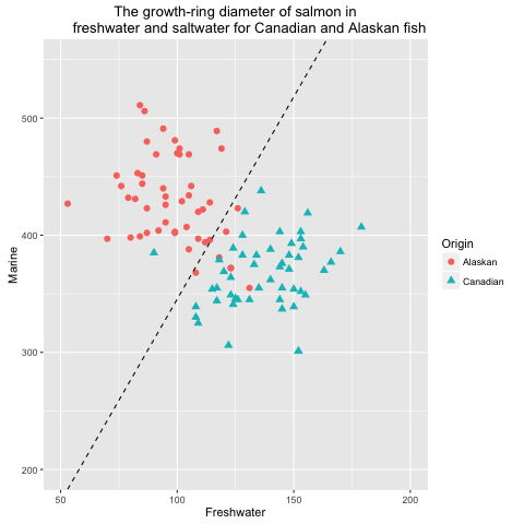
Fig 6. Visualisation of classified salmon data using perceptrons
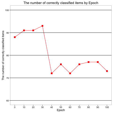
Fig 7. Changes of the classification accuracy of perceptrons regarding to the number of epoch
References
Hebb, D. O. (1949). The Organization of Behavior. New York, NY, USA: John Wiley. Johnson, R. A. & Wichern, D. W. (2007, April). Applied Multivariate Statistical Analysis (6th ed.). London, UK: Pearson.
Krizhevsky, A., Sutskever, I., & Hinton, G. E. (2012, December). ImageNet Classification with Deep Convolutional Neural Networks. In F. Pereira, C. J. C. Burges, L. Bottou, & K. Q. Weinberger (Eds.), Advances in Neural Information Processing Systems (Stateline, NV, USA) (pp. 1097– 1105). NIPS ’12. Red Hook, NY, USA: Curran Associates. Retrieved from http ://papers.nips.cc/paper/4824-imagenet-classification-with-deep-convolutional-neural-networks.pdf
McCulloch, W. S. & Pitts, W. (1943, December). A Logical Calculus of the Ideas Immanent in Nervous Activity. The Bulletin of Mathematical Biophysics, 5(4), 115–133. Retrieved from 10.1007/bf02478259 Minsky, M. & Papert, S. (1969). Perceptrons. Cambridge, MA, USA: MIT press.
Rosenblatt, F. (1958, November). The Perceptron: a Probabilistic Model for Information Storage and Organization in the Brain. Psychological Review, 65(6), 386–408.