Table of Contents
II. From single-layer perceptrons to multilayer perceptrons
1. Introduction
In Part 1, we have discussed about threshold functions and perceptrons, the most simplest form of neural nets that is capable of learning but still constrained when it is only applicable to linear separable problems. In Part 2, our topic is the second form of neural networks, particularly feedforward multilayer perceptrons. In details, we will discuss: (i) why this type of networks can solve nonlinear classification tasks, (ii) why it is called feedforward, and (iii) how a multilayer perceptron can learn from the data.
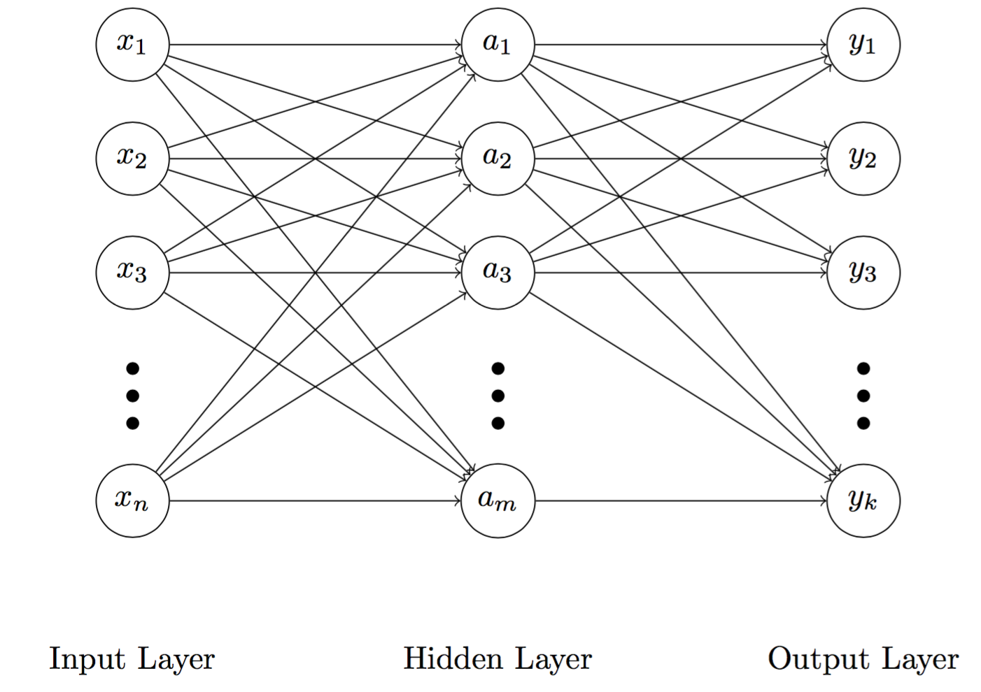
Fig 1. Illustration of a multilayer perceptron
A typical feedforward artificial neural network has three different layers, including the input layer, the hidden layer, and the output layer (Figure 1). The second layer is intuitively called the hidden layer because it is masked by both the input and output layers. Whilst a node in the input and output layers is corresponding to a predictor and an output, nodes in the hidden layer employ an activation function, about which we will discuss later.
2. Activation function
Activation function enables nonlinear mapping between inputs and outputs of neurons. Figure 2 illustrates examples of activation functions by which we can have nonlinear output from an initial linear input. Activation functions has three essentially attributes. First, they are nonlinear. Second, their outputs are constrained within certain boundaries, for example $(0, 1)$ in the case of the logistic functions, making them appropriate for classification tasks where we are only interested in nominal outputs. Finally, they are continually differentiable. This characteristic allows to optimise the cost function using differential equations, such as gradient descent.
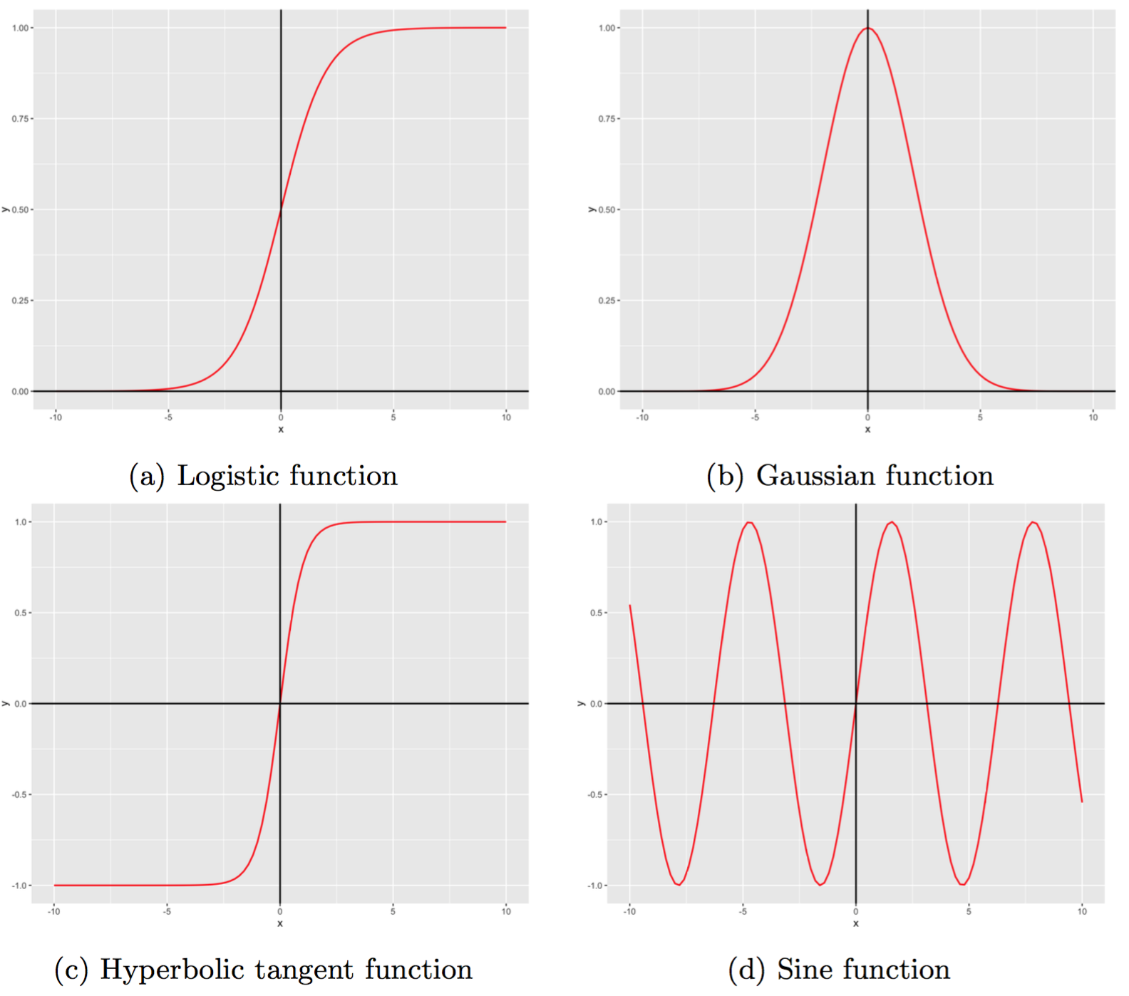
Fig 2. Examples of activation functions
3. Inside hidden neurons
To understand how feedforward operates, it is important to understand the internal characteristic of hidden nodes. Similar to threshold neurons, a hidden neuron consists of a transfer function $\Sigma$ and an activation function $\varphi$ (instead of a threshold function in case of a threshold neuron). Mathematically, $\Sigma$ is given by
\[\begin{aligned} \Sigma & = \Theta^T \mathbf{x} \\ \varphi & = \varphi(\Sigma) = \varphi(\Theta^T \mathbf{x}) \end{aligned}\]where $\Theta = \begin{bmatrix} \theta_1 & \theta_2 \cdots \theta_n \end{bmatrix}^T$ is a vector of weights. Thus, we can calculate the output $y$ of the hidden node in Figure 3 by
\[y = \varphi(\Theta^T \mathbf{x})\]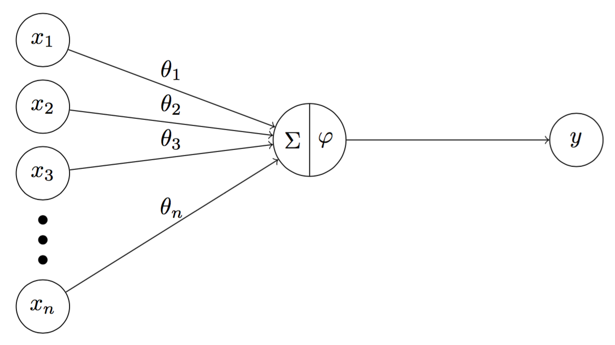
Fig 3. A hidden neuron consists of a transfer function $\sum$ and an activation function $\varphi$
4. Feedforward
The term feedforward is devised to help distinguish from another kinds of neural networks where connections between nodes can be circles, such as recurrent neural networks. In feedforward neural networks, connections flows straightforwardly from the input layers to the output layer.
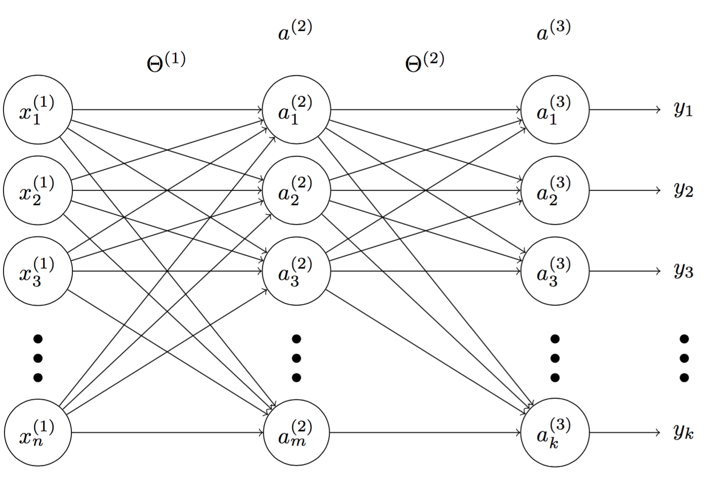
Fig 4. A multilayer perceptron
In Figure 4, we have multilayer perceptrons with $n$ inputs, $m$ activation nodes and $k$ outputs. Denote $\mathbf{\Theta^{(1)}}$ and $\mathbf{\Theta^{(2)}}$ matrices of weights between inputs-hidden layers and hidden-output layers. $\mathbf{\Theta^{(1)}}$ and $\mathbf{\Theta^{(2)}}$ are given by
\[\mathbf{\Theta^{(1)}} = \begin{bmatrix} \Theta^{(1)}_1 \\ \Theta^{(1)}_2 \\ \Theta^{(1)}_3 \\ \cdots \\ \Theta^{(1)}_{m} \end{bmatrix} = \begin{bmatrix} \theta^{(1)}_{11} & \theta^{(1)}_{12} & \theta^{(1)}_{13} & \cdots & \theta^{(1)}_{1n} \\ \theta^{(1)}_{21} & \theta^{(1)}_{22} & \theta^{(1)}_{23} & \cdots & \theta^{(1)}_{2n} \\ \theta^{(1)}_{31} & \theta^{(1)}_{32} & \theta^{(1)}_{33} & \cdots & \theta^{(1)}_{3n} \\ \cdots & \cdots & \cdots & \cdots & \cdots \\ \theta^{(1)}_{m1} & \theta^{(1)}_{m2} & \theta^{(1)}_{m3} & \cdots & \theta^{(1)}_{mn} \\ \end{bmatrix}\] \[\mathbf{\Theta^{(2)}} = \begin{bmatrix} \Theta^{(2)}_1 \\ \Theta^{(2)}_2 \\ \Theta^{(2)}_3 \\ \cdots \\ \Theta^{(2)}_{m} \end{bmatrix} = \begin{bmatrix} \theta^{(2)}_{11} & \theta^{(2)}_{12} & \theta^{(2)}_{13} & \cdots & \theta^{(2)}_{1m} \\ \theta^{(2)}_{21} & \theta^{(2)}_{22} & \theta^{(2)}_{23} & \cdots & \theta^{(2)}_{2m} \\ \theta^{(2)}_{31} & \theta^{(2)}_{32} & \theta^{(2)}_{33} & \cdots & \theta^{(2)}_{3m} \\ \cdots & \cdots & \cdots & \cdots & \cdots \\ \theta^{(2)}_{m1} & \theta^{(2)}_{m2} & \theta^{(2)}_{m3} & \cdots & \theta^{(2)}_{km} \\ \end{bmatrix}\]where $\Theta^{(1)}_j$ $(j = 1,…, m)$ is a weight vector of connections from $a^{(2)}_j$ to $\mathbf{x^{(1)}}$ and $\Theta^{(2)}_i$ $(i = 1,…, k)$ is a weight vector of connections from $a^{(3)}_i $ to $\mathbf{a^{(2)}}$.
From $\mathbf{\Theta^{(1)}}$ and $\mathbf{\Theta^{(2)}}$, we can calculate $\mathbf{a^{(2)}}$ and $\mathbf{a^{(3)}}$ respectively
\[\begin{aligned} \mathbf{a^{(2)}} & = \varphi (\mathbf{\Theta^{(1)}} \cdot \mathbf{x^T}) \qquad \qquad \qquad \, \, {\mathbf{(1)}} \\ \mathbf{a^{(3)}} & = \varphi (\mathbf{\Theta^{(2)}} \cdot \mathbf{a^{(2)}}) \qquad \qquad \qquad {\mathbf{(2)}} \end{aligned}\]Finally, the output $\mathbf{y}$ is
\[\mathbf{y} = \mathbf{a^{(3)}}\]Example Suppose we want to classify a set of data points generated by XOR operation.
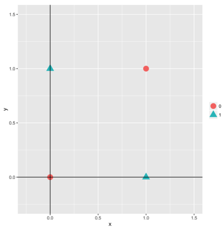
Fig 5. Graph of data points given in Table 1
Figure 5 is a graph of XOR data points. Look at the graph, we can intuitively see that we cannot classify them using linear model, such as perceptron. Instead, in this example, we will use the feedforward neural network model. Particularly, we can classify such dataset using a feedforward neural network with 3 inputs, 3 hidden neurons, and 1 output (Figure 6). Note that $x^{(1)}_0$ is a bias unit.
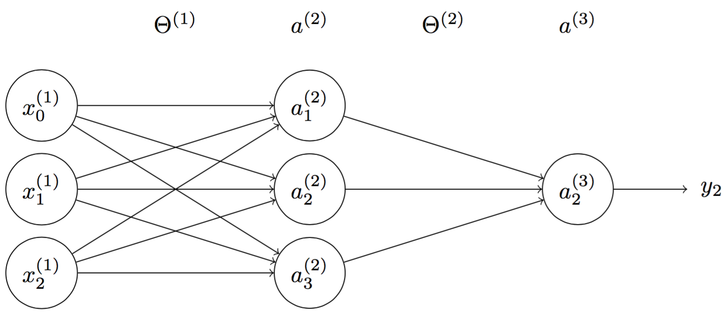
Fig 6. A sample multilayer perceptron to classify XOR gate
Suppose we have
\[\mathbf{\Theta^{(1)}} = \begin{bmatrix} -3.9628723 & -8.481784 & 7.694714 \\ 2.9412002 & -7.297706 & 9.293525 \\ 0.2272201 & 4.008646 & 3.443932 \end{bmatrix}\] \[\mathbf{\Theta^{(2)}} = \begin{bmatrix} 14.52022 & -13.81069 & 7.022461 \\ \end{bmatrix}\]We begin with the first observation $x_1 = 1, x_2 = 1$, and set bias unit $x_0 = 1$. Thus, $\mathbf{x} = \begin{bmatrix} 1 & 1 & 1 \end{bmatrix}$. From (1) and (2), we can obtain $\mathbf{a^{(2)}}$
\[\begin{aligned} \mathbf{a^{(2)}} & = \varphi (\mathbf{\Theta^{(1)}} \cdot \mathbf{x^T}) \\ & = \varphi \Bigg( \begin{bmatrix} -3.9628723 & -8.481784 & 7.694714 \\ 2.9412002 & -7.297706 & 9.293525 \\ 0.2272201 & 4.008646 & 3.443932 \end{bmatrix} \begin{bmatrix} 1 \\ 1 \\ 1 \end{bmatrix} \Bigg) \\ &\approx \varphi \Bigg( \begin{bmatrix} -4.749942 \\ 4.937019 \\ 7.679798 \end{bmatrix} \Bigg) \approx \begin{bmatrix} 0.008577978 \\ 0.992875171 \\ 0.999538145 \end{bmatrix} \end{aligned}\]From $\mathbf{a^{(2)}}$, we now can obtain $\mathbf{a^{(3)}}$
\[\begin{aligned} \mathbf{a^{(3)}} & = \varphi (\mathbf{\Theta^{(2)}} \cdot \mathbf{a^{(2)}}) \\ &= \varphi \Bigg( \begin{bmatrix} 14.52022 & -13.81069 & 7.022461 \\ \end{bmatrix} \begin{bmatrix} 0.008577978 \\ 0.992875171 \\ 0.999538145 \end{bmatrix} \Bigg) \\ &\approx \varphi (\begin{bmatrix} -6.568518 \end{bmatrix}) \approx 0.001401908 \end{aligned}\]Thus we have $y = 0.001401908 \approx 0$ for $x_1 = 1, x_2 = 1$. Repeat the whole process with new inputs, we can obtain $y = 0.9988276$ with $x_1 = 1, x_2 = 0$, $y = 0.9992674$ with $x_0 = 1, x_2 = 1$, and finally $y = 0.0001311898$ with $x_0 = 0, x_2 = 0$.
5. Backpropagation
Suppose we have
- $e_j$ is the error at the neuron $j$.
- $d_j$ is the desire output at neuron $j$.
- $E$ is the error of the neuron $j$ for all inputs of a class $C$.
- $s_j$ is the sum of outputs $y_i$ of neurons from the previous layer $i$.
- $y_j$ is the output of neuron $j$.
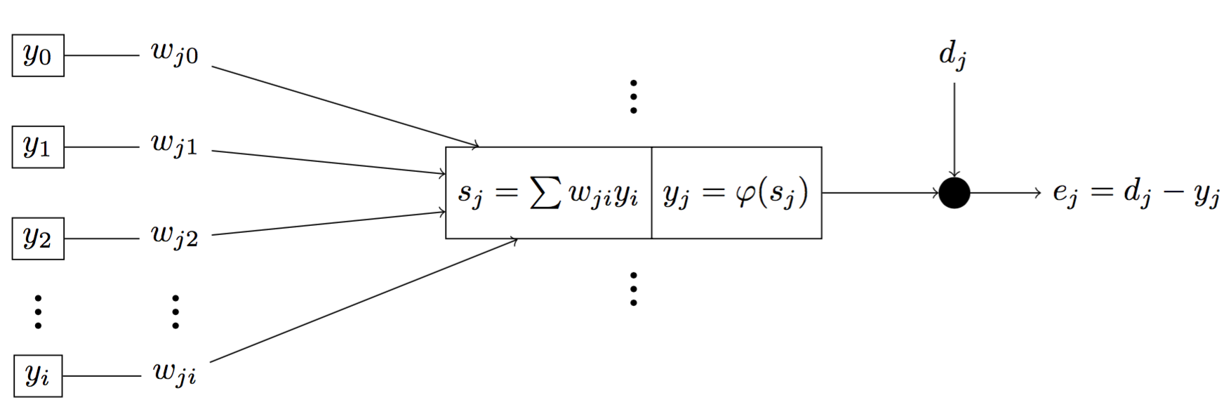
Fig 7. Graph of signal flow of a neuron j in the network
We can represent them mathematically
\[\begin{aligned} e_j = d_j - y_j \qquad \qquad \qquad {\mathbf{(1)}} \\ E = \frac{1}{2} \sum_{j \in C} e^2_j \qquad \qquad \qquad {\mathbf{(2)}} \\ s_j = \sum_{i = 0} w_{ji} y_i \qquad \qquad \qquad {\mathbf{(3)}} \\ y_j = \varphi(s_j) \qquad \qquad \qquad {\mathbf{(4)}} \end{aligned}\]Our goal is to find $\Delta w_{ji}$ such that we can find the local minima of $E$
\[\Delta w_{ji} = - \eta \frac{\partial E}{\partial w_{ji}} \qquad \qquad \qquad {\mathbf{(5)}}\]Thus, to find $\Delta w_{ji}$, we need to find $\frac{\partial E}{\partial w_{ji}}$. Apply the chain-rule, we can have
\[\frac{\partial E}{\partial w_{ji}} = \frac{\partial E}{\partial e_j} \cdot \frac{\partial e_j}{\partial y_j} \cdot \frac{\partial y_j}{\partial s_j} \cdot \frac{\partial s_j}{\partial w_{ji}} \qquad \qquad \qquad {\mathbf{(6)}}\]Each component in ${\mathbf{(6)}}$ can be resolved as
\[\begin{aligned} {\mathbf{(1)}} \quad &\Rightarrow \quad \frac{\partial E}{\partial e_j} = e_j \\ {\mathbf{(2)}} \quad &\Rightarrow \quad \frac{\partial e_j}{\partial y_j} = -1 \\ {\mathbf{(3)}} \quad &\Rightarrow \quad \frac{\partial y_j}{\partial s_j} = \varphi ' (s_j) \\ {\mathbf{(4)}} \quad &\Rightarrow \quad \frac{\partial s_j}{\partial w_{ji}} = y_i \\ \end{aligned}\]Based on that, we can rewrite ${\mathbf{(6)}}$
\[{\mathbf{(6)}} \quad \Rightarrow \quad \frac{\partial E}{\partial w_{ji}} = - e_j \cdot \varphi ' (s_j) \cdot y_i \qquad \qquad \qquad {\mathbf{(7)}}\]Using ${\mathbf{(7)}}$, we also rewrite ${\mathbf{(5)}}$ by
\[{\mathbf{(5)}} \quad \Rightarrow \quad \Delta w_{ji} = \eta \frac{\partial E}{\partial w_{ji}} = \eta \cdot e_j \cdot \varphi ' (s_j) \cdot y_i \qquad \qquad \qquad {\mathbf{(8)}}\]Suppose we have \(\begin{aligned} \delta_j &= - \frac{\partial E}{\partial s_j} \\ &= - \frac{E}{\partial e_j} \cdot \frac{\partial e_j}{\partial y_j} \cdot \frac{\partial y_j}{\partial s_j} \\ &= e_j \cdot \varphi ' (s_j) \qquad \qquad \qquad \qquad \qquad {\mathbf{(9)}} \end{aligned}\)
Plug ${\mathbf{(9)}}$ into ${\mathbf{(8)}}$, we have
\[{\mathbf{(7)}} + {\mathbf{(8)}} \quad \Rightarrow \quad \Delta w_{ji} = \eta \cdot {\delta_j} \cdot y_i \qquad \qquad \qquad {\mathbf{(10)}}\]Now we have a beautiful form of local gradient $\Delta w_{ji}$, but unfortunately, we still cannot calculate $\Delta w_{ji}$ because $\delta_j$, although in such a beautiful form, still cannot be easily calculated. Thus, our next goal is to find a computable form of $\delta_j$.
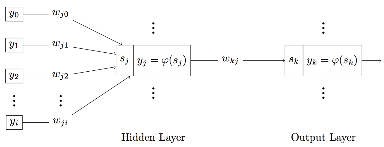
Fig 8. Graph of signal flow when neuron j is a hidden neuron, neuron k is an output neuron
For a neuron $j$, there are two cases. It is either a output neuron or a hidden. If neuron $j$ is a output neuron, we can easily compute $\delta_j$ because we already known the desired output $d_j$ and predicted output $y_j$. Thus,
\[\delta_j = e_j \cdot \varphi ' (s_j) = (d_j - y_j) \cdot \varphi ' (s_j) \qquad \qquad \qquad {\mathbf{(11)}}\]On the other hand, if neuron $j$ is a hidden neuron, we can have
\[\begin{aligned} \delta_j &= - \frac{\partial E}{\partial s_j} = - \frac{\partial E}{\partial y_j} \cdot \frac{\partial y_j}{\partial s_j} \\ &= - \frac{\partial E}{\partial y_j} \cdot \varphi ' (s_j) \qquad \qquad \qquad {\mathbf{(12)}} \end{aligned}\]Suppose neuron $k$ is the output neuron, we have
\[E = \frac{1}{2} \sum_{k \in C} e^2_k \qquad \qquad \qquad {\mathbf{(13)}}\] \[\begin{aligned} {\mathbf{(13)}} \quad \Rightarrow \quad \frac{\partial E}{\partial y_j} &= \sum_{k} e_k \cdot \frac{\partial e_k}{\partial y_j} \\ &= \sum_{k} e_k \cdot \frac{\partial e_k}{\partial s_k} \cdot \frac{\partial s_k}{\partial y_j} \qquad \qquad \qquad {\mathbf{(14)}} \end{aligned}\]Note that $e_k = d_k - y_k = d_k - \varphi (s_k)$, thus we have
\[\frac{\partial e_k}{\partial s_k} = - \varphi ' (s_k) \qquad \qquad \qquad {\mathbf{(15)}}\]Also, for neuron $k$, we can have $s_k = \sum w_{kj} \cdot y_j$, thus,
\[\frac{\partial s_k}{\partial y_j} = w_{kj} \qquad \qquad \qquad {\mathbf{(16)}}\]Plug ${\mathbf{(15)}}$ and ${\mathbf{(16)}}$ into ${\mathbf{(14)}}$, we have
\[{\mathbf{(13)}} + {\mathbf{(14)}} + {\mathbf{(15)}} \quad \Rightarrow \quad \frac{\partial E}{\partial y_j} = - \sum_k e_k \cdot \varphi ' (s_k) \cdot w_{kj} \qquad \qquad {\mathbf{(16)}}\]And because neuron $k$ is an output neuron, from ${\mathbf{(11)}}$ we have
\[{\mathbf{(10)}} \quad \Rightarrow \quad \delta_k = e_k \cdot \varphi ' (s_k) \qquad \qquad \qquad {\mathbf{(18)}}\]Thus, plug ${\mathbf{(18)}}$ into ${\mathbf{(17)}}$, we have
\[{\mathbf{(17)}} + {\mathbf{(18)}}\quad \Rightarrow \quad \frac{\partial E}{\partial y_j} = - \sum_k \delta_k \cdot w_{kj} \qquad {\mathbf{(19)}}\]Thus,
\[\begin{aligned} {\mathbf{(12)}} + {\mathbf{(19)}} \quad \Rightarrow \quad \delta_j &= - \frac{\partial E}{\partial y_j} \cdot \varphi ' (s_j) \\ &= \varphi ' (s_j) \sum_k \delta_k \cdot w_{kj} \qquad {\mathbf{(20)}} \end{aligned}\]Finally, we find a comprehensive way to calculate $\delta_j$ when neuron $j$ is either a hidden neuron or output neuron in ${\mathbf{(11)}}$ and ${\mathbf{(20)}}$.
- If neuron $j$ is an output neuron, $\delta_j = e_j \cdot \varphi ‘ (s_j) = (d_j - y_j) \cdot \varphi ‘ (s_j) $
- If neuron $j$ is a hidden neuron, $\delta_j = \varphi ‘ (s_j) \sum \delta_k \cdot w_{kj}$ where $\delta_k$ is of output neuron $k$
5.1. Error signal
Recall that to make our equations mathematically convenient, we have defined $\delta_j = - \frac{\partial E}{\partial s_j}$. But doing so is not just for mathematical convenience, in fact, $\delta_j$ does carry meanings in its own definition. In the network, $\delta_j$ is called the error signal at neuron $j$, and it indicates how much the error at neuron $j$ varies with respect to the input $s_j$. If we can determine $\delta_j$, which of course we can by using backpropagation, we can subsequently decide new weight values $w$ that can lower the total error $E$.
Backward transmission In contrast to feedforward where signals flow from the input layer to the output layer, in backpropagation, signals are transferred in the opposite direction, from the output layer back to the input layers. In particular, the transferred signals is error signals. And that is why the algorithm is named backpropagation in the first place.
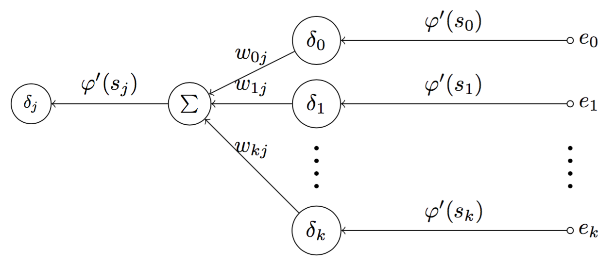
Fig 9. Graph of error signal flow when neuron j is a hidden neuron
Figure 9 depicts a graph of error signal flow for a hidden neuron $j$. First, at the output layer, the error signal $e_k$ of the output neuron $k$ is computed. Since neuron $k$ is an output neuron, the error signal of neuron $k$ can be computed by $\delta_k = e_k \cdot \varphi ‘ (s_j)$. By repeating the process for another output neurons, we can subsequently have $\delta_0$, $\delta_1$, … of the output layer. For every computed error signals, we have a corresponding weights $w_{0j},…, w_{kj}$, we can compute $\sum = \sum {w_{kj}}{\delta_k}$. Finally, we will have $\delta_j = \varphi ‘ (s_j) \sum {w_{kj}}{\delta_k}$.
5.2. Summary of backpropagation
Backpropagation algorithm can be applied generally by following steps:
- Use feedforward to compute corresponding sums of inputs and weights $s$ of every neuron and predicted outputs $y_k$ considering neuron $k$ as output neurons.
- Compute the error signals $\delta$ for every neurons. If neuron $j$ is an output neuron, then $\delta_j = e_j \cdot \varphi ‘ (s_j) = (d_j - y_j) \cdot \varphi ‘ (s_j) $. If neuron $j$ is a hidden neuron, then $\delta_j = \varphi ‘ (s_j) \sum \delta_k \cdot w_{kj}$ where $\delta_k$ is of output neuron $k$.
- Update network weights by $\Delta w_{ji} = \eta \cdot \delta_j y_i$.
6. Experiment
In this section, we will implement a neuron network of three inputs, three hidden neurons and one output to classify the XOR data. The experiment is conducted using R.
During this experiment, we tried to use different initial weight values $w$, and as a result, sometimes the optimisation of error rate did not converge even after 1000 epochs. Figure 10 depicts two scenarios, one when the error rate drop nearly to 0 after 1000 epochs, one does not. Thus, we can conclude that backpropagation, because employing gradient descent to optimise weights, does not promise that it can find local minima of the error rate. Thus, it is required to have gradient checking method to measure the process.
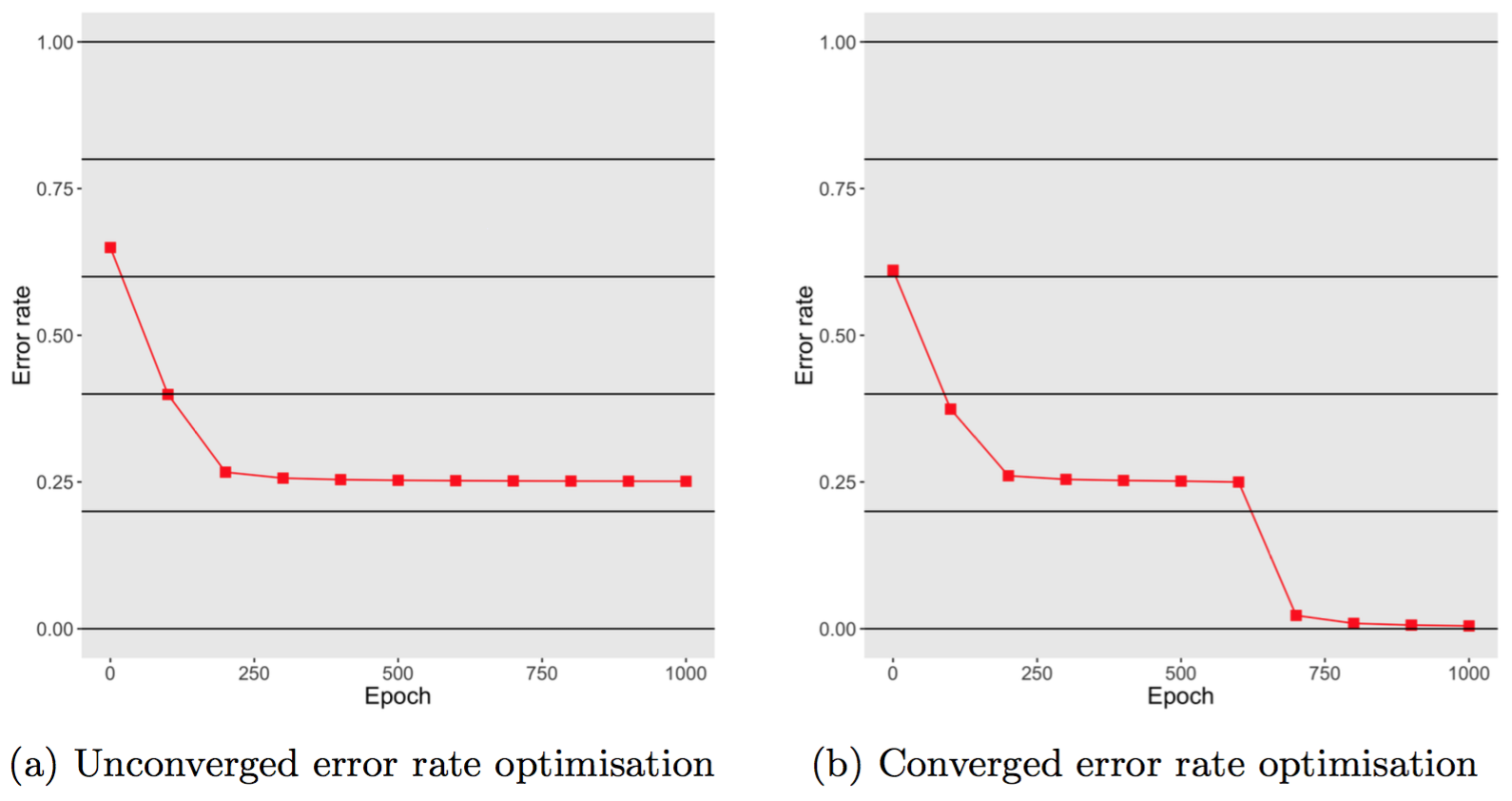
Fig 10. Error rates varies according the number of epochs