Table of Contents
- III. Posterior probabilities with softmax and cross-entropy
III. Posterior probabilities with softmax and cross-entropy
1. Softmax
The softmax function, also known as the normalised exponential, is a function that maps a vector of real values to a vector whose values are normalised in the range (0, 1) and sum of them equals to 1 (Bishop, 2006). The function is given by
\[\varphi (s_j) = \frac{e^{s_j}}{\sum_{k=1}^{K} e^{s_k}}\]where $K$ is the number of possible outcomes. In multiclass classification models, $K$ is the number of classes that we want to classify.
By analysing the formula of the softmax function, we can see why the softmax function allows to obtain normalised exponential values.
- The numerator and denominator of the function are always greater than 0, thus, the output vector of the function is always positive.
- The denominator of the function is the sum of $K$ corresponding classes, hence, the output values of the function are in the range (0, 1) and sum up to 1.
Example Suppose we have a input vector $v$ of 4 elements, $v = \begin{bmatrix} 1 \ 2 \ 3 \ 4 \end{bmatrix}$, we can have the transformed vector $\varphi (v)$ by using the softmax, $\varphi (v) = \begin{bmatrix} 0.032 \ 0.087 \ 0.236 \ 0.644 \end{bmatrix}$.
Relationship with logistic regression Softmax and logistic regression have a relationship where softmax is a generalised version of logistic regression. In case we use softmax as the activation function of the output layer for a binary classification task, softmax behaves similarly to logistic regression.
To demonstrate that mathematically, suppose we have a neural networks where we use logistic regression to perform a binary classification task. In the output layer of 1 single neuron, we would have the output $y$ given by
\[\begin{align} y = \frac{1}{1 + e^{-s_1}} = \frac{1}{1 + \frac{1}{e^{s_1}}} &= \frac{e^{s_1}}{1 + e^{s_1}} \\ &= \frac{e^{s_1}}{e^{s_0} + e^{s_1}} \tag*{$s_0 = 0$}\\ &= \frac{e^{s_1}}{\sum_{k=0}^{1}e^{s^k}} \end{align}\]This equation demonstrates that a neural network with the softmax output layer of 2 neurons, where the weight of one output neuron always equals 0, behaves similarly to the neural network of the logistic regression output layer of 1 single neuron.
2. Cross-entropy
The term cross-entropy origins from information theory and is later applied to machine learning for model training. In training neural networks, the cross-entropy cost function is given by
\[J(\theta) = -\frac{1}{m} \bigg[ \sum_{j=1}^{k} 1\{y^{(i)} = j\} \, \log \frac{e^{s_j}}{\sum_{i = 1}^{k} e^{s_k}} \bigg]\]where $k$ is the number of output neurons.
Note that in the equation above, $1{.}$ is the indicator function, such that \(1\{ true \, statement \} = 1\) and \(1\{ false \, statement \} = 0\).
Intuition In information theory, the concept of entropy was firstly introduced by (Shannon, 2001). Shannon’s entropy refers to the contained information in a message, basically represented by bits.
An intuitive example is that suppose we need to inform our friends whenever we see a car or a bicycle crossing by our place. We can only use binary numbers and hence, for each kind of vehicles, we would use different bit sequences. We might want to encode our bit sequences in a way that we can send messages effectively. Should we encode them the same? No, we should not because the number of bicycles on the street is certainly smaller than the number of cars, hence, we would certainly broadcast bit sequences of car more frequent than bit sequences of bicycle. Those optimal number of bits we choose to encode are called entropy, which can given by
\[H(x) = \sum_{i} x_i \log \frac{1}{x_i} = - \sum_{i} x_i \log x_i\]In our example, suppose the number of cars is 256 times higher than the number of bicycles. We would have
\[b_{car} = \log_2 \frac{1}{256 * p_{bicycle}} = \log_2 \frac{1}{256} + \log_2 \frac{1}{p_{bicycle}} = b_{bicycle} - 8\]This result indicates that we should encode the bit sequences of car using 8 bits less than the number of bit sequences of bicycle.
Recently, we are able to find the optimal number of bits or entropy by exploiting the underlying factual distribution of cars and bicycles on the street. What if we are clueless about that distribution and thus, we would guess. By using that guess, we would subsequently encode our bit sequences in a different manner, such that
\[H(x, \hat{x}) = \sum_{i} x_i \log \frac{1}{\hat{x}_i} = - \sum_{i} x_i \log \hat{x}_i\]In this case, we would encode our bits using guessing values \(\hat{x}_i\), where $x$ is the desired values. And the number of bits we encode using $H(x, \hat{x})$ is known as cross-entropy. We can intuitively see that our cross-entropy is always higher than entropy, and they only equal to each other if we can make perfect guesses.
2.1. Neural network training
2.1.1. Output layer
Suppose we have
- $e_j$ is the error at the neuron $j$.
- $d_j$ is the desire output at neuron $j$.
- $E$ is the error of the neuron $j$ for all inputs of a class $C$.
- $s_j$ is the sum of outputs $y_i$ of neurons from the previous layer $i$.
- $y_j$ is the output of neuron $j$.
In the MSE cost function, we define $e_j = d_j - y_j$ and $E = \frac{1}{2} \sum e^2_j$. In the cross-entropy cost function, we will adjust both of them, such that,
\[\begin{align} e_j & = - \big[ d_j \, \ln y_j + (1 - d_j) \ln (1 - y_j) \big] \tag{1} \\ E & = \sum_{j \in C} e_j & \tag{2} \\ s_j & = \sum_{i = 0} w_{ji} y_i \tag{3} \\ y_j & = \varphi(s_j) \tag{4} \end{align}\]Thus, we can have
\[\begin{align} \frac{\partial E}{\partial w_{ji}} = \frac{\partial E}{\partial e_j} \cdot \frac{\partial e_j}{\partial y_j} \cdot \frac{\partial y_j}{\partial s_j} \cdot \frac{\partial s_j}{\partial w_{ji}} \tag{5} \end{align}\]Each component in ${(6)}$ can be resolved as
\[\begin{align} {(2)} \quad &\Rightarrow \quad \frac{\partial E}{\partial e_j} = 1 \\ {(1)} \quad &\Rightarrow \quad \frac{\partial e_j}{\partial y_j} = - \frac{d - y}{y(1-y)} \\ {(4)} \quad &\Rightarrow \quad \frac{\partial y_j}{\partial s_j} = \varphi ' (s_j) \\ {(3)} \quad &\Rightarrow \quad \frac{\partial s_j}{\partial w_{ji}} = y_i \\ \end{align}\]Based on that, we can rewrite ${(5)}$
\[\begin{align} {(5)} \quad \Rightarrow \quad \frac{\partial E}{\partial w_{ji}} = - \bigg[ \frac{d - y}{y(1-y)} \cdot \varphi ' (s_j) \cdot y_i \bigg] \tag{6} \end{align}\]We already know that the activation function has many types, however, when $\varphi (\cdot)$ is the sigmoid function and the cost function is cross-entropy, a beautiful and interpretable form of the gradient of training error, which we will see, appears.
As said, when $\varphi (\cdot)$ is the sigmoid function, we can obtain $\varphi ‘ (\cdot) = \big[ \varphi (\cdot) (1 - \varphi (\cdot) \big]$. Thus, ${(6)}$ will become
\[\begin{align} {(6)} \quad \Rightarrow \quad \frac{\partial E}{\partial w_{ji}} & = - \bigg[ \frac{d - y}{y(1-y)} \cdot \varphi(s_j) (1-\varphi(s_j)) \cdot y_i \bigg] \\ &= - \bigg[ \frac{d - \varphi (s_j))}{\varphi (s_j) ( 1 - \varphi (s_j))} \cdot \varphi(s_j) (1-\varphi(s_j)) \cdot y_i \bigg] \\ &= - \bigg[ (d - y_j) \cdot y_i \bigg] \tag{7} \end{align}\]${(7)}$ demonstrates how the weights change with respect to the cross-entropy cost function. By examining ${(7)}$, we can see the changing of the weights in the network is solely dependent on the difference between the actual output and the output of the network. That observation can lead to a more interesting conclusion that the speed of learning of our neurons is decided by the degree of the mistake they make. The bigger the mistake, the faster our neurons learn.
2.1.2. Hidden layer
${(7)}$ is the gradient of the training error at the output layer. Next, we will find out $\frac{\partial E}{\partial w_{ji}}$ in case neuron $j$ is the hidden neuron. Again, we have
\[\begin{align} \frac{\partial E}{\partial w_{ji}} = \sum_{k=1}^{nout} \frac{\partial E}{\partial e_k} \cdot \frac{\partial e_k}{\partial y_k} \cdot \frac{\partial y_k}{\partial s_k} \cdot \frac{\partial s_k}{\partial y_j} \cdot \frac{\partial y_j}{\partial s_j} \cdot \frac{\partial s_j}{\partial w_{ji}} \tag{8} \end{align}\] \[\begin{align} \frac{\partial E}{\partial e_k} &= \frac{\partial}{\partial e_k} {e_k} = 1 \tag{9} \\ \frac{\partial e_k}{\partial y_k} &= - \frac{d - y_k}{y_k(1-y_k)} \tag{10} \\ \frac{\partial y_k}{\partial s_k} &= \frac{\partial}{\partial s_k} \varphi (s_k) = \varphi (s_k) \big[1-\varphi (s_k) \big] \tag{11} \\ \frac{\partial s_k}{\partial y_j} &= \frac{\partial}{\partial y_j} \sum w_{kj} y_j = w_{kj} \tag{12} \\ \frac{\partial y_j}{\partial s_j} &= \frac{\partial}{\partial s_j} \varphi (s_j) = \varphi (s_j) \big[1-\varphi (s_j) \big] \tag{13} \\ \frac{\partial s_j}{\partial w_{ji}} &= \frac{\partial}{\partial w_{ji}} \sum w_{ji} y_i = y_i \tag{14} \\ \end{align}\]Plug (9), (10), (11), (12), (13), (14) into (8), we would have
\[\begin{align} \frac{\partial E}{\partial w_{ji}} &= \sum_{k=1}^{nout} - \frac{d - y_k}{y_k(1-y_k)} \cdot \varphi (s_k) \big[1-\varphi (s_k) \big] \cdot w_{kj} \cdot \varphi (s_j) \big[1-\varphi (s_j) \big] \cdot y_i \\ &= \sum_{k=1}^{nout} - (d-y_k) \cdot w_{kj} \cdot \varphi (s_j) \big[ 1-\varphi (s_j)\big] \cdot y_i \\ &= \sum_{k=1}^{nout} \frac{\partial E}{\partial w_{kj}} \cdot w_{kj}(1-y_j)y_i \tag{15} \end{align}\]3. Softmax and sigmoid in neural networks
In this section, we will see how we can train a neural network of 3 layers that uses softmax in the output layer, and sigmoid in the hidden layer (Figure 1). Compare to neural networks that use sigmoid function in the output layer, this network, with the support of softmax function, will be able to produce posterior probability in multi-class classification tasks.
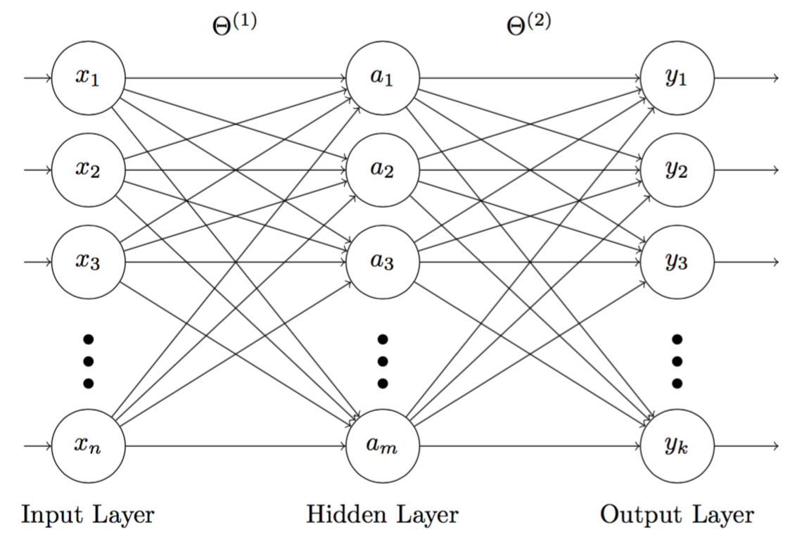
Figure 1: 3-layer neuron network, where the hidden nodes $a_j$ $(j = 1,..., m)$ use sigmoid and the output nodes $y_i$ $(i = 1,..., k)$ uses softmax
3.1. Derivative of the softmax function
\[f(x) = \frac{g(x)}{h(x)} \Rightarrow f'(x) = \frac{g'(x)h(x) - h'(x)g(x)}{[h(x)]^2}\] \[\begin{align} g(s_j) &= e^{s_j} \Rightarrow \frac{\partial g}{\partial s_i} = \begin{cases} 0 & \text{if } i \neq j \\ e^{s_j} & \text{if } i = j \end{cases} \\ h(s_j) &= \sum_{k=1}^{N} e^{s_k} \Rightarrow \frac{\partial h}{\partial s_i} = e^{s_j} \tag*{for both $i = j$ and $i \neq j$} \end{align}\]- If $i \neq j$
- If $i = j$
3.2. Training
3.2.1. Output layer
Suppose we have
- $E$ is the error of the neuron $j$ for all inputs of a class $C$.
- $s_j$ is the sum of outputs $y_i$ of neurons from the previous layer $i$.
- $y_j$ is the output of neuron $j$.
In the MSE cost function, we define $e_j = d_j - y_j$ and $E = \frac{1}{2} \sum e^2_j$. In the cross-entropy cost function, we will adjust both of them, such that,
\[\begin{align} E & = - \sum_{j=1}^{nclass} t_j \log y_j \\ s_j & = \sum_{i = 0} w_{ji} y_i \\ y_j & = \varphi(s_j) \end{align}\] \[\begin{align} \frac{\partial E}{\partial w_{ji}} = \frac{\partial E}{\partial s_j} \cdot \frac{\partial s_j}{\partial w_{ji}} \end{align}\]Each component in ${(6)}$ can be resolved as
\[\begin{align} \frac{\partial E}{\partial s_j} &= - \frac{\partial}{\partial s_j} \bigg[ t_j \log y_j + \sum_{j \neq i}^{nclass} t_j \log y_j \bigg] \\ &= - \frac{t_j}{y_j} \frac{\partial y_j}{\partial s_j} - \sum_{i \neq j} \frac{t_i}{y_i} \frac{\partial y_i}{\partial s_j} \\ &= - \frac{t_j}{y_j} y_j (1-y_j) + \sum_{i \neq j} \frac{t_i}{y_i} y_i y_j \\ &= -t_j (1-y_j) + \sum_{i \neq j} t_i y_j \\ &= -t_j + t_j y_j + \sum_{i \neq j} t_i y_j \\ &= -t_j + \sum_{i = 1} t_i y_j \\ &= -t_j + y_j \sum_{i = 1} t_i \\ &= y_j - t_j \tag*{because $\sum_{j = 1} t_j = 1$} \end{align}\] \[\begin{align} \frac{\partial s_j}{\partial w_{ji}} = y_i \end{align}\] \[\begin{align} \frac{\partial E}{\partial w_{ji}} = \frac{\partial E}{\partial s_j} \cdot \frac{\partial s_j}{\partial w_{ji}} = (y_j - t_j) y_i \end{align}\]3.2.2 Hidden layer
\[\begin{align} \frac{\partial E}{\partial s_k} = y_k - t_k \end{align}\] \[\begin{align} \frac{\partial s_k}{\partial y_j} = \frac{\partial \sum w_{kj}y_j}{\partial y_j} = w_{kj} \end{align}\] \[\begin{align} \frac{\partial y_j}{\partial s_j} = y_j (1 - y_j) \end{align}\] \[\begin{align} \frac{\partial s_j}{\partial w_{ji}} = y_i \end{align}\] \[\begin{align} \frac{\partial E}{\partial w_{ji}} &= \frac{\partial E}{\partial s_k} \cdot \frac{\partial s_k}{\partial y_j} \cdot \frac{\partial y_j}{\partial s_j} \cdot \frac{\partial s_j}{\partial w_{ji}} \\ &= (y_k - t_k) \cdot (w_{kj}) \cdot y_j (1-y_j) \cdot y_i \end{align}\]4. Experiment
Up to now, we already know how to train 3-layer neural network having the sigmoid function in the hidden layer, and the softmax function in the output layer. In this section, we will use derived formulas to train that kind of network for a multi-category classification task.
4.1. Data description
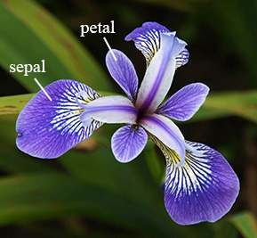
Figure 2: An Iris flower with labels
The dataset used in this experiment is the Iris flower dataset (Anderson, 1935; Fisher, 1936). This dataset contains 50 samples of 3 species of Iris (i.e., setosa, virginica, and versicolor). All of 3 species are characterised by 4 features, including the sepal length, sepal width, petal length, and petal width. Figure 2 is a typical Iris flower and Figure 3 provides a visual description of those features.
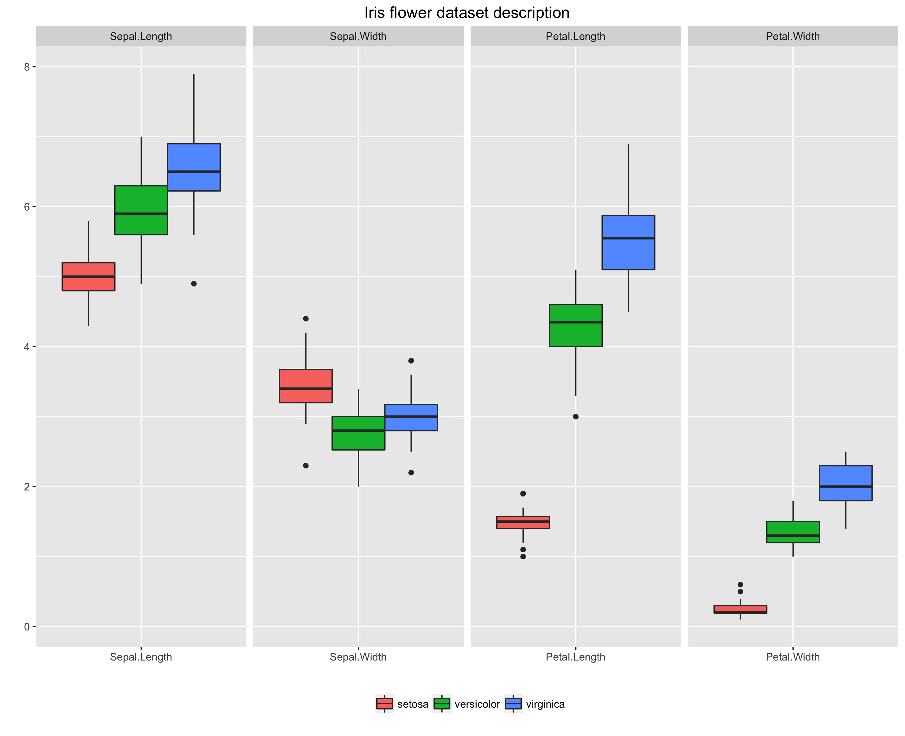
Figure 3: Iris flower dataset description of 4 features: sepal length, sepal width, petal length, and petal width
4.2. Classification model
The classification model used in this experiment is a 3-layer neuron network:
- Input layer: 5 inputs including $x_0$ is the bias unit and $x_1, x_2, x_3, x_4$ are for 4 features.
- Hidden layer: 5 sigmoid activation units $a_j$ $(j = 0,…,4)$.
- Output layer: 3 softmax outputs $y_j$ $(j = 1, 2, 3)$ according to 3 predicted classes.
Figure 4 is a model representation of the network and Figure 5 is a signal flow model of the network.
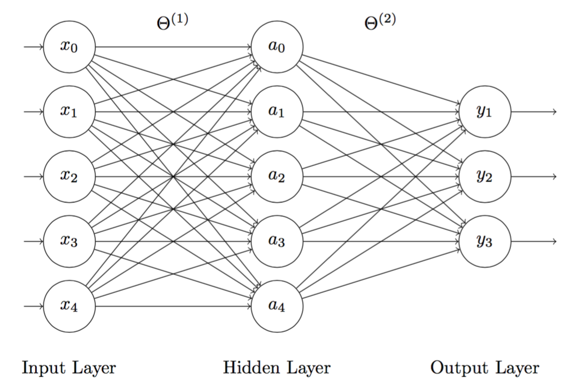
Figure 4: 3-layer neuron network, where the hidden nodes $a_j$ $(j = 1,..., 4)$ use sigmoid and the output nodes $y_i$ $(i = 1,..., 3)$ uses softmax. Note that the bias term $x_0$ equals to 1. $\Theta^{(1)}$ and $\Theta^{(2)}$ are weights.
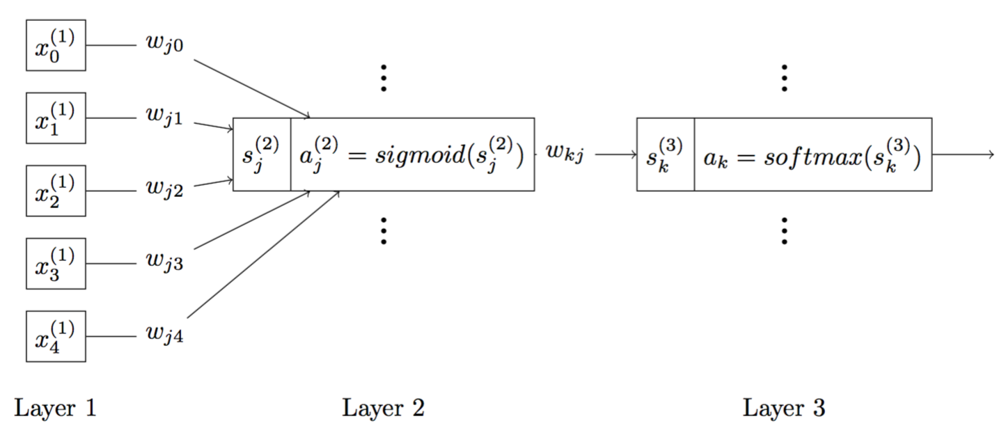
Figure 5: A description of signal flow of the neural network
4.3. Results
As said, what we can expect from this model is the posterior probability. An example of the model output is that suppose we have a particular observation belongs to 1st class (e.g., setosa), the encoded output of that observation in this experiment would be \(Y = \begin{bmatrix} 1 \\ 0 \\ 0 \end{bmatrix}\). Corresponding with that desired output $Y$, the expected prediction of the classification model would be like \(\hat{Y} = \begin{bmatrix} 0.6609379 \\ 0.1009062 \\ 0.2381559 \end{bmatrix}\), where 0.6609379 represents the probability that this particular observation would be setosa is 66.09%.
Figure 6 and 7 are the visual reports of the experiment. In this experiment, we divided the data into 80% for training and 20% for testing. Note that:
-
The learning converges early. Both Figure 7 demonstrates that both the training and testing accuracy reach their optimal points somewhere before 5000 epochs. When analysing experiment procedures, we can conclude that this early convergence can be achieved due to:
- Optimal initialisation of weights we initialised weights with mean equals 0 and standard devidation equals $1/\sqrt[2]{n_w}$ where $n_w$ is the number of connecting weights to the neuron. By initialising the weights by this method, we have better chance in avoiding the learning saturation of the model (Haykin, 2009).
- Maximisation of learning for every epoch, we shuffled the training data, which makes the learning process very healthy (Haykin, 2009).
-
Overfitting is controlled very well Thanks to L2 regularisation, it seems that overfitting is avoided in the experiment. Figure 7 shows that the accuracy of the testing set is essentially better than the accuracy of the training set. Besides, we can also observe that the accuracy of the testing set slightly correlates with the accuracy of the training set in this experiment.
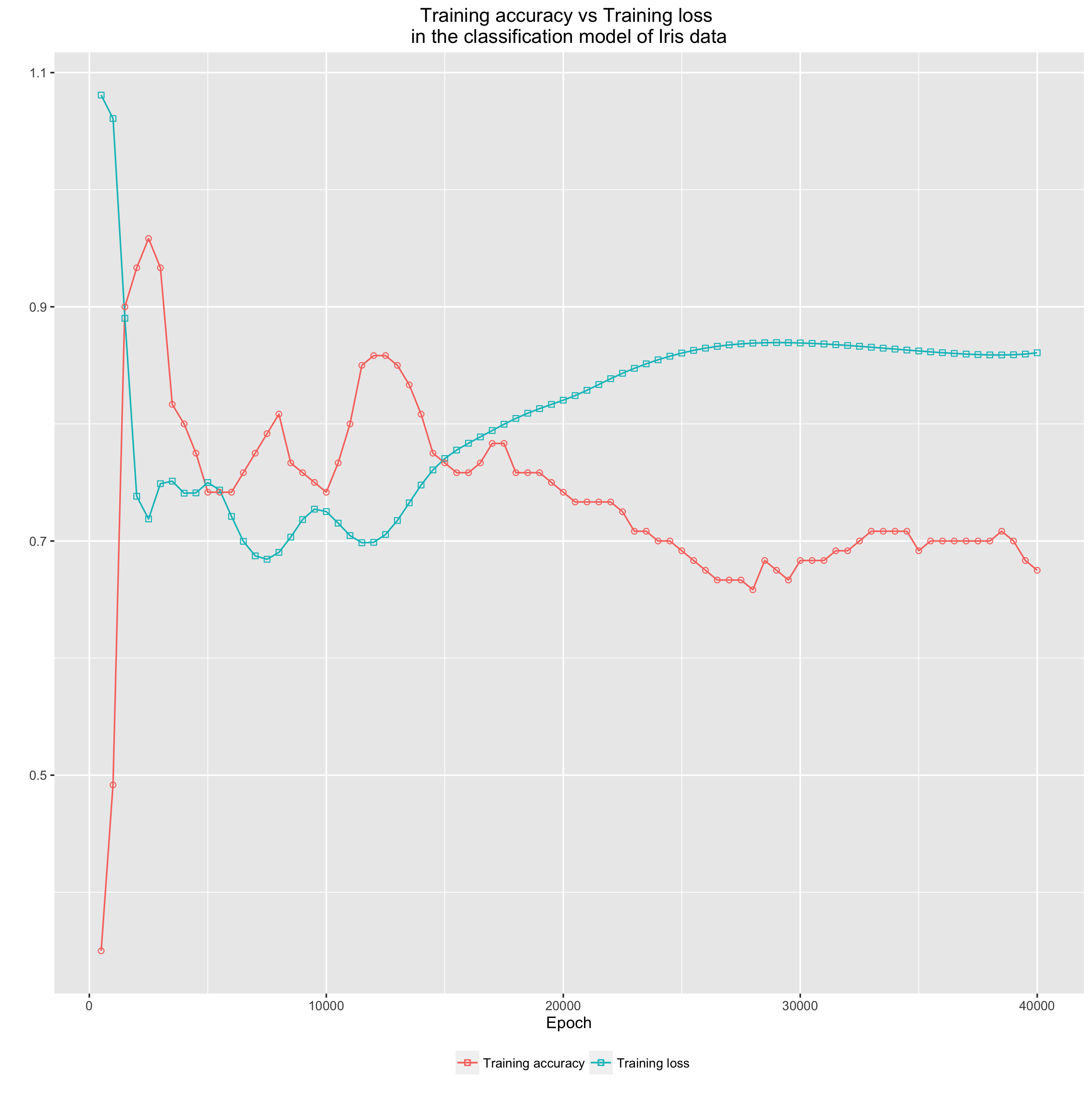
Figure 6: Accuracy vs loss in the Iris flower classification model
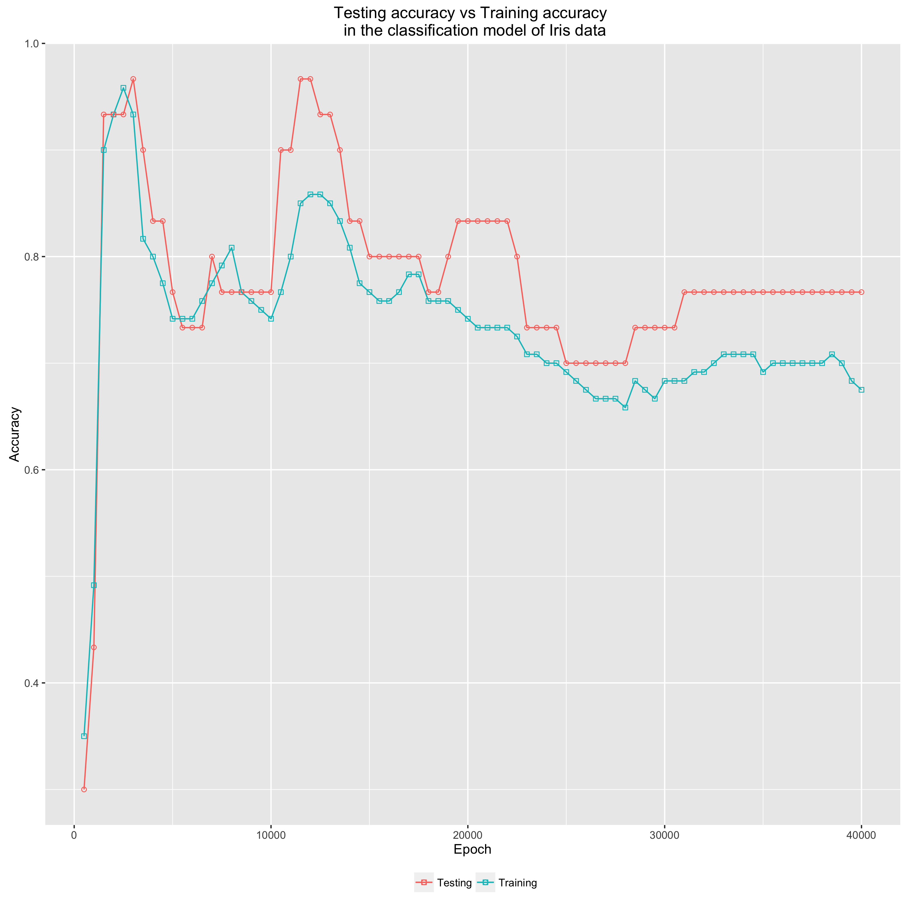
Figure 7: Training accuracy vs Testing accuracy in the Iris flower classification model
The code snippet of the experiment implementation in R.
References
Anderson, E. (1935, September). The Species Problem in Iris. Annals of the Missouri Botanical Garden, 23(3), 457–469. doi:10.2307/2394164
Bishop, C. M. (2006). Pattern Recognition and Machine Learning. Berlin, Germany: Springer.
Fisher, R. A. (1936, September). The use of multiple measurements in taxonomic problems. Annals of Eugenics, 7(2), 179–188. doi:10.1111/j.1469-1809. 1936.tb02137.x
Haykin, S. (2009). Neural Networks and Learning Machines (3rd ed.). Upper Saddle River, NJ, USA: Pearson.
Shannon, C. E. (2001, July). A Mathematical Theory of Communication. Bell Labs Technical Journal, 27(4), 623–656. doi:10.1002/j.1538-7305.1948. tb01338.x