Table of Contents
III. Regularisation in neural networks
1. Introduction
Overfitting prefers to the problem, where a machine learning model is able to perform (very) well on the training data, but (very) poorly on the unseen data. There are 3 typical methods to conquer overfitting:
- Increasing the amount of the data This method is considered as the most effective technique to prevent overfitting. Unfortunately, data is not always available, and often expensive to acquire.
- Reducing the dimension of the data This method is technically preferred as _feature selection} in machine learning, where we only use a subset of features to build the model.
- Adding regularisation term We can use regularisation to add additional complexity to the cost function, which can help to prevent overfitting.
Suppose $J_0$ is the original cost function of the model, we can have the modified cost function $J$ of the model by adding the regularisation component. The new cost function is given by
\begin{equation} J = J_0 + \lambda R(\theta) \end{equation}
where $R(\theta)$ is the regularisation term, whose strength can be governed by $\lambda$.
There are many regularisation techniques, however, within the scope of this writing, we will primarily focus on two particular techniques, namely $\ell$-$1$ and $\ell$-$2$ regularisation.
2. Benefits of regularisation
It is already known that the purpose of the minimisation of the cost function is to find the set of coefficients $\theta$ that produce the cheaper cost function. However, it is often that our optimisation could result in an ``exploded’’ set of coefficients with high variance, making our model poorly fit to the unseen data. In other words, we would say our model is overfitted.
In our case, our model demonstrates traits of overfitting because its coefficients have high variance. This symptom exists because we impose no restriction on coefficients, allowing them to freely obtain any possible values that simply will give minimal value to the cost function. Hence, to reduce overfitting, we might want to regularise coefficients while learning. Our idea is mathematically demonstrated by
\begin{align} \operatorname*{arg\,min}_\theta J(\theta) \quad s.t. \quad R(\theta) \leq 0 \end{align}
The expression $(2)$ remarks the idea of finding possible values of $\theta$ at which the cost function $J(\theta)$ is minimal while satisfying $g(\theta) \leq 0$.
Although $(1)$ and $(2)$ seems different, they are equivalent to each other. We can show that by rewriting $(2)$ using Lagrange multipliers in the following section.
2. Lagrange multipliers
Before we show how to rewrite and optimise $(2)$ using Lagrange multipliers, we will briefly discuss it. In a nutshell, Lagrange multipliers is a mathematical method used to solve equality/inequality constrained optimisation of differentiable functions. In this section, we will discuss the naive intuition behind Lagrange multipliers and how it can be used to solve optimisation problems. For more explanations focusing on intuition, it is advised to read (Klein, 2004; Smith, 2004).
2.1. Equality constraints
Suppose we have two distinct functions $f(\theta)$ and $g(\theta)$ and we want to find extreme values of $f(\theta)$ while satisfying $g(\theta) = 0$. The geometric intuition behind Lagrange multipliers is that we can only find extreme points that satisfy conditions when two contours of $f$ and $g$ are tangent (not intersection). When they are tangent, the gradient vectors of $f$ and $g$ are parallel, which can be expressed by
\begin{align} \nabla f(\theta) &= \lambda \nabla g(x) \end{align}
where $\lambda$ is the Lagrangian multipliers.
The equation $(3)$ is the centre idea. The Lagrangian equation can be written based on that
\begin{align} \mathcal{L}(\theta, \lambda) = f(\theta) - \lambda g(\theta) \end{align}
From $(4)$ we can find extreme points by solving the following equation
\begin{align} \nabla \mathcal{L}(\theta, \lambda) = 0 \end{align}
2.2. Inequality constraints
In the previous section, we have the condition that $g(\theta) = 0$. When we are no longer interested in the usual constraint $g(\theta) = 0$, but $g(\theta) \leq 0$ or $g(\theta) \geq 0$, we need to apply Lagrange multipliers in a slightly different way.
Similar to $(3)$, we still have
\begin{align} \nabla f(\theta) &= \lambda \nabla g(\theta) \end{align}
But now we have additional constraints for $\lambda$
\[\begin{align} g(\theta) \geq 0 \Rightarrow \lambda \geq 0 \\ g(\theta) \leq 0 \Rightarrow \lambda \leq 0 \end{align}\]Given $(7)$ and $(8)$, we can find the extreme points that satisfy the inequality constraints by solving the following equations
\[\begin{align} \nabla \mathcal{L}(\theta, \lambda) = 0 \\ \text{if} \quad g(\theta) \geq 0, \lambda \geq 0 \\ \text{if} \quad g(\theta) \leq 0, \lambda \leq 0 \end{align}\]2.3. Constrained cost function minimization
Until now we already see how Lagrangian multipliers can be used to solve optimisation problems of differential functions with either equality or inequality constraints. Now we will see how Lagrangian can be applied to a particular case, where we want to optimise the cost function $J(\theta)$ while constraining coefficients $\theta$ by certain conditions. We can elaborate our idea by the expression
\begin{align} \operatorname*{arg\,min}_\theta J(\theta) \quad &s.t. \quad R(\theta) \leq c \end{align}
where $c$ is a constant. By moving everything to one side, we can have
\begin{align} (10) \Leftrightarrow \operatorname*{arg\,min}_\theta J(\theta) \quad &s.t. \quad c - R(\theta) \geq 0 \end{align}
Now we can write a Lagrangian of $(11)$. Note that $\lambda$ is now constrained by $\lambda \geq 0$ in the same manner as $(8)$.
\[\begin{align} \mathcal{L}(\theta, \lambda) &= J(\theta) - \lambda (c - R(\theta)) \\ \Leftrightarrow \mathcal{L}(\theta, \lambda) &= J(\theta) + \lambda \big[R(\theta) - c \big] \end{align}\]Compare $(1)$ and $(13)$, we can see that the regularised cost function is essentially a constrained optimisation problem, and $\lambda$ - the regularisation parameter to govern the regularisation term - is indeed the Lagrangian multiplier.
3. $\ell$-$1$ and $\ell$-$2$ regularisations
$\ell$-$1$ regularisation is the sum of the absolute value of weights, which can be given by
\begin{align} R(\theta) = \lVert \theta \rVert_1 = \sum_{i=1}^{n} | \theta_i| \end{align}
$\ell$-$2$ regularisation is _the sum of the square of weights}, which can be given by
\begin{align} R(\theta) = \lVert \theta \rVert_2^2 = \sum_{i=1}^{n} \theta_i^2 \end{align}
Characteristics of $\ell$-$1$ and $\ell$-$2$ regularisation techniques in comparison.
Sparsity $\ell$-$1$ exhibits a trait that it tends to create a sparse coefficient vector, whereas $\ell$-$2$ does not. In case of $\ell$-$1$ regularisation, we can imagine that the shape of the constraint function in 2D plane would be a rectangular, and in most of the time, the contour of the cost function $J_0$ would be tangent to the constraint at a corner, which would be the extreme point that $J_0$ is minimal while the constraint is satisfied (Figure 1). At that extreme point, we easily see that one of the coefficient is 0 (in a 2D plane). That may explain why $\ell$-$1$ tends to create sparse vectors. In contrast, in $\ell$-$2$ regularisation, because the constraint function does not have sharp points, generally the tangent point will not be on an axis. Thus, the coefficients in $\ell$-$2$ regularisation will be non-zero.
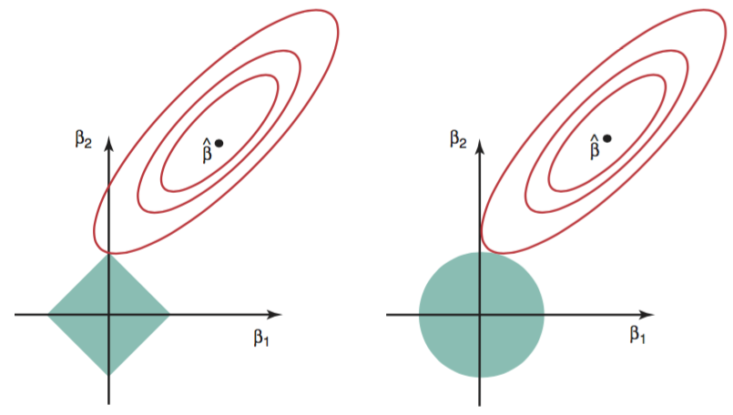
Figure 1: Visualisation of the error and constraint functions of l-1 (left) and l-2 (right) (James, Witten, Hastie, & Tibshirani, 2013)
Feature selection $\ell$-$1$ regularisation is also considered as a feature selection method, because it leads to sparse coefficient vectors (i.e., if a feature has the zero value of weight, it is removed from the model).
4. Experiment
In this experiment, we will use the Iris data again to demonstrate how regularisation helps constraint coefficients, which results in a regulated cost function and less overfitting model. Figure 2, 3 and 4 evidently show that without the regularisation term, the cost function and the accuracy of both training and testing are severely vacillating.
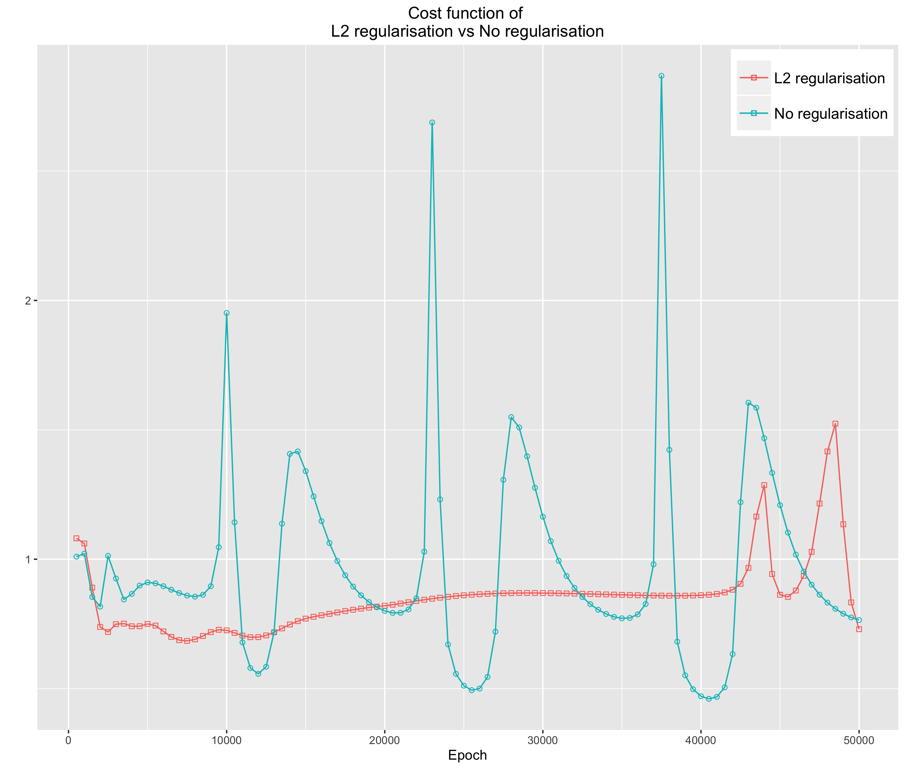
Figure 2: The cost function with l-2 regularisation and none
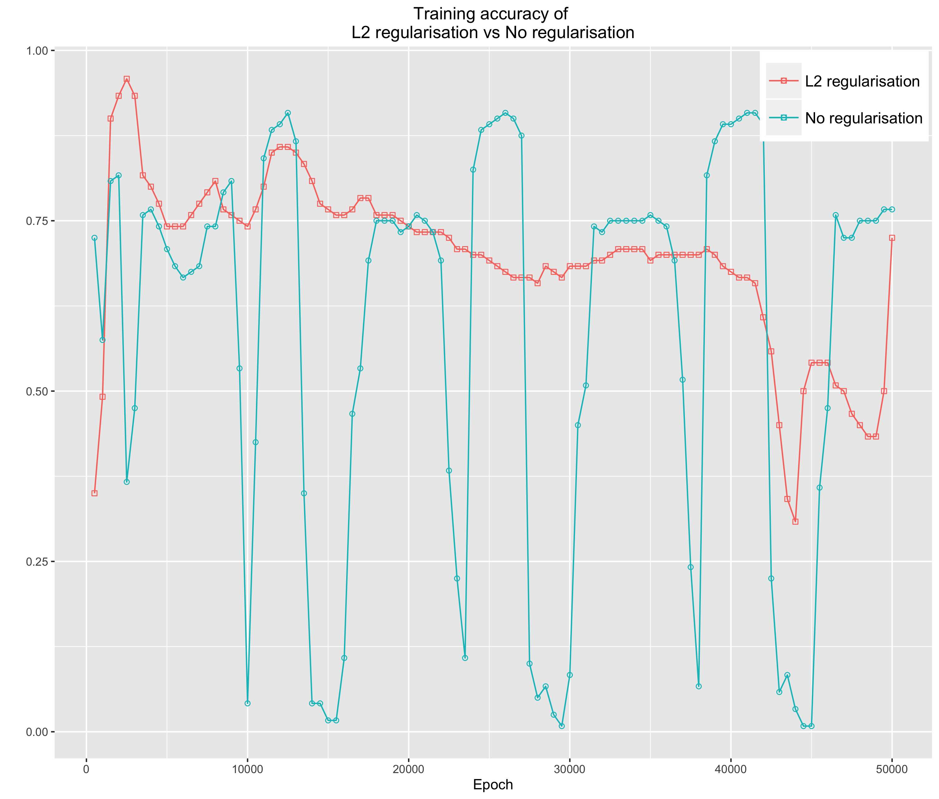
Figure 3: The training accuracy with l-2 regularisation and none
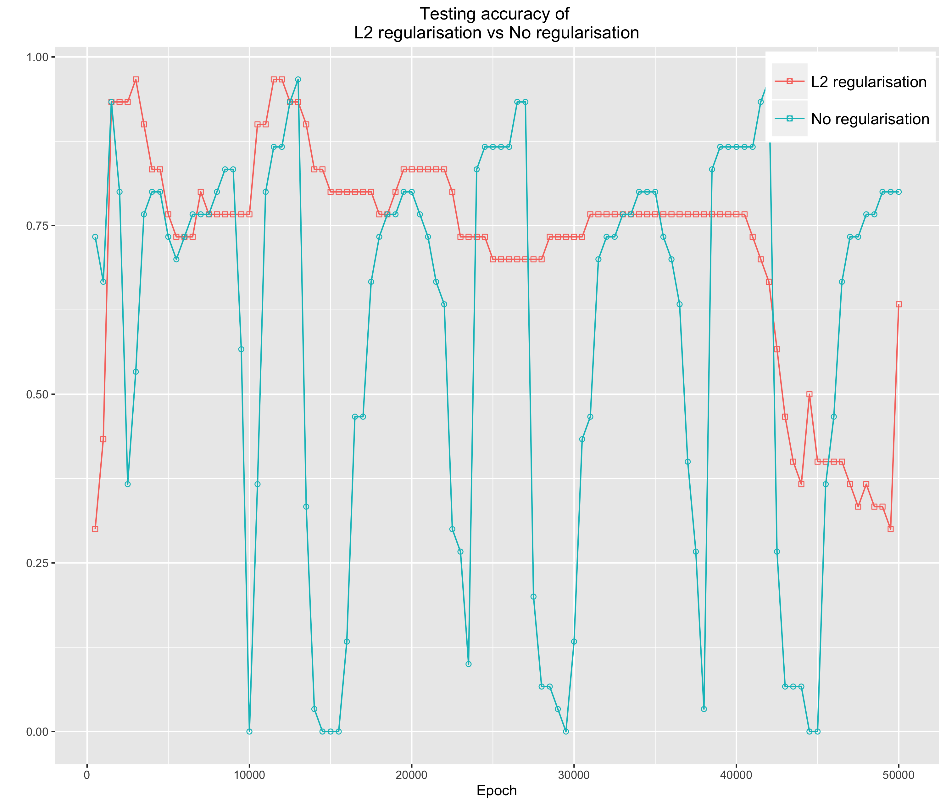
Figure 4: The testing function with l-2 regularisation and none
Below is the R code implementation of the experiment.
References
James, G., Witten, D., Hastie, T., & Tibshirani, R. (2013, June). An Introduction to Statistical Learning. Berlin, Germany: Springer.
Klein, D. (2004). Lagrange Multipliers Without Permanent Scarring. Online. Retrieved from http://www.cs.berkeley.edu/∼klein/papers/lagrange- multipliers.pdf
Smith, B. T. (2004, June). Lagrange Multipliers Tutorial in the Context of Support Vector Machines. Online. Retrieved from http://www.engr.mun. ca/∼baxter/Publications/LagrangeForSVMs.pdf