Digit classification using MNIST dataset is kind of “hello world” exercise to Neural Net and Deep Learning (DL) – i.e. an introductory example to demonstrate neural networks. Although I plant to blog a more interesting DL modeling in the future, I still think it is always nice to have a “hello world” example to start off with.
I - Load packages
At the start, we load necessary packages that we will use in this project.
import tensorflow as tf
import numpy as np
from tensorflow import keras
import matplotlib.pyplot as plt
import pandas as pd

np.random.seed(1)
NUMBER_OF_CLASSES = 10
EPOCHS = 500
BATCH_SIZE = 256
VALIDATION_SPLIT = .2
II - Load and Process the Dataset
1. Observe the dataset
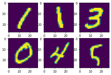
According to the dataset description, the data files contain gray-scale images in terms of pixel values, of hand-written digits from 0 to 9. Each image has the size of 28 x 28 pixels (height x width).
To explore the dataset, we first load the data conveniently using keras.
# Load MNIST dataset
(X_train, Y_train), (X_test, Y_test) = keras.datasets.mnist.load_data()
Let’s see some examples of the dataset.
idx = [3, 6, 7, 1, 9, 100]  # Example indices
fig, axs = plt.subplots(2, 3)
axs[0, 0].imshow(X_train[idx[0]])
axs[0, 1].imshow(X_train[idx[1]])
axs[0, 2].imshow(X_train[idx[2]])
axs[1, 0].imshow(X_train[idx[3]])
axs[1, 1].imshow(X_train[idx[4]])
axs[1, 2].imshow(X_train[idx[5]])
<matplotlib.image.AxesImage at 0x7f46d816e8e0>
Next, we are going to explore our dataset:
print("X_train shape:", X_train.shape)
print("Y_train shape:", Y_train.shape)
print("Y_train classes: %i classes" % np.unique(Y_train).size)
print("X_test shape:", X_test.shape)
print("Y_test shape:", Y_test.shape)

print("Number of training examples:", X_train.shape[0])
print("Number of testing examples: ", X_test.shape[0])
print("Number of unique classes: %i classes" % np.unique(Y_train).size)
print("Each image is of size: %i x %i" % X_train.shape[1:3])
X_train shape: (60000, 28, 28)
Y_train shape: (60000,)
Y_train classes: 10 classes
X_test shape: (10000, 28, 28)
Y_test shape: (10000,)
Number of training examples: 60000
Number of testing examples:  10000
Number of unique classes: 10 classes
Each image is of size: 28 x 28
The dimensions of X_train shows that our training dataset has 60k training examples of 28x28 pixels. Besides, our test dataset, which is X_test shows that we have 10k test examples of the same 28x28 pixels.
2. Reshape the dataset
Prior to feeding the training and test dataset to the network, it is necessary to flatten and standardize examples. Here, flattening refers to reshaping each image of 28x28 pixels from 2-dimensions (corresponding to height and width) to a 1-dimension vector of 784 pixels.
X_train_preprocessed = X_train.reshape(X_train.shape[0], -1)
X_test_preprocessed = X_test.reshape(X_test.shape[0], -1)
print("Flatten shape of X_train: ", X_train_preprocessed.shape)
print("Flatten shape of X_test: ", X_test_preprocessed.shape)
Flatten shape of X_train:  (60000, 784)
Flatten shape of X_test:  (10000, 784)
For Y_train and Y_test, it is a bit more complicated because currently, both are in 1-D array. We need to process them using one-hot encoding and transpose so that they are in the same form as X_train_preprocessed and X_test_preprocessed.
Y_train_preprocessed = keras.utils.to_categorical(Y_train, NUMBER_OF_CLASSES)
Y_test_preprocessed = keras.utils.to_categorical(Y_test, NUMBER_OF_CLASSES)
print("Current shape of Y_train_preprocessed:", Y_train_preprocessed.shape)
print("Current shape of Y_test_preprocessed:", Y_test_preprocessed.shape)
Current shape of Y_train_preprocessed: (60000, 10)
Current shape of Y_test_preprocessed: (10000, 10)
So far, we have reshaped all of our arrays into a desired shape, that is, each column represents a data example while each row represent features (for X_train_preprocessed and X_test_preprocessed) or one-hot encoding class (for Y_train_preprocessed and Y_test_preprocessed).
3. Standardize the dataset
Since the maximum value of each pixel in an image is 255, it is a common practice to divide the dataset by a value of 255 to scale it to [0, 1] range.
X_train_preprocessed = X_train_preprocessed / 255
X_test_preprocessed = X_test_preprocessed / 255
III - 2-Layer Neural Network Model Using Keras
Using tf.keras to construct and train a neural network is suprisingly straightforward and elegance. In this example, we build a 2-layer neural network using the Sequential model of keras. Particularly, in the hidden layer, we have 32 nodes and use ReLU as our activation function; in the output layer, we have 10 outputs corresponding to 10 digits and use softmax as our activation function to output the prediction probabilities for each node.
# Build the model
mnist_model = keras.models.Sequential(name="simple_2_layer_mnist")
mnist_model.add(keras.Input(shape=(784,)))
mnist_model.add(keras.layers.Dense(units=32, activation='relu'))
mnist_model.add(keras.layers.Dense(units=10, activation='softmax'))
# Compile the model
mnist_model.compile(optimizer='SGD',
              loss='categorical_crossentropy',
              metrics=['accuracy'])
mnist_model.summary()
Model: "simple_2_layer_mnist"
_________________________________________________________________
Layer (type)                 Output Shape              Param #
=================================================================
dense_2 (Dense)              (None, 32)                25120
_________________________________________________________________
dense_3 (Dense)              (None, 10)                330
=================================================================
Total params: 25,450
Trainable params: 25,450
Non-trainable params: 0
_________________________________________________________________
# Fit the model
history = mnist_model.fit(X_train_preprocessed, Y_train_preprocessed,
         batch_size=BATCH_SIZE,
         epochs=EPOCHS,
         verbose=2,
         validation_split=VALIDATION_SPLIT)
# Evaluate the model with X_test and Y_test of 10k examples
mnist_model.evaluate(X_test_preprocessed, Y_test_preprocessed)
313/313 [==============================] - 0s 758us/step - loss: 0.1134 - accuracy: 0.9666

[0.11341889947652817, 0.9666000008583069]
IV - Model History
After fitting the model to the training set, keras function .fit() outputs an object called history object. This particular object provides a record of all the loss and our chosen metrics. We can make use of this object to see how our model performed in training and validation sets.
# Convert this object to a dataframe
df_loss_acc = pd.DataFrame(history.history)
df_loss_acc.describe()
| loss | accuracy | val_loss | val_accuracy | |
|---|---|---|---|---|
| count | 500.000000 | 500.000000 | 500.000000 | 500.000000 |
| mean | 0.150920 | 0.957532 | 0.168337 | 0.953066 |
| std | 0.118133 | 0.032421 | 0.086647 | 0.020004 |
| min | 0.074324 | 0.461812 | 0.117592 | 0.721750 |
| 25% | 0.090917 | 0.950839 | 0.124928 | 0.950729 |
| 50% | 0.117783 | 0.966271 | 0.141163 | 0.959417 |
| 75% | 0.173927 | 0.974198 | 0.181851 | 0.964333 |
| max | 1.804684 | 0.979146 | 1.325913 | 0.967000 |
# Extract to two separate data frames for loss and accuracy
df_loss = df_loss_acc[['loss', 'val_loss']]
df_loss = df_loss.rename(columns={'loss': 'Loss', 'val_loss': 'Validation Loss'})
df_acc = df_loss_acc[['accuracy', 'val_accuracy']]
df_acc = df_acc.rename(columns={'accuracy': 'Accuracy', 'val_accuracy': 'Validation Accuracy'})

# Plot the data frames
df_loss.plot(title='Training vs Validation Loss', figsize=(10, 6))
df_acc.plot(title='Training vs Validation Accuracy', figsize=(10, 6))
<AxesSubplot:title={'center':'Training vs Validation Accuracy'}>
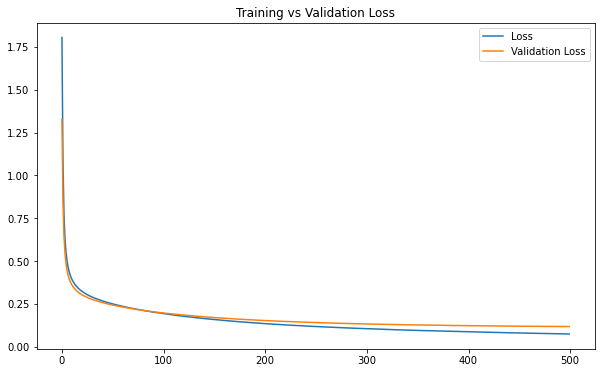
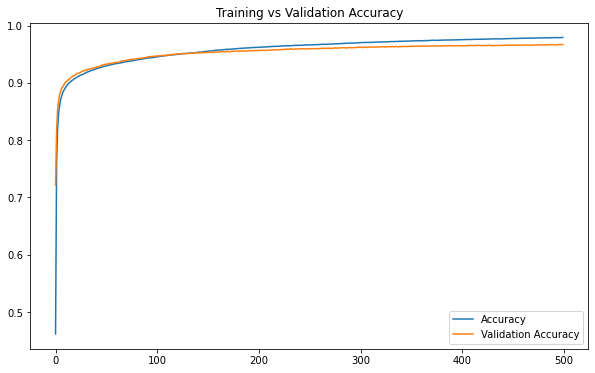
It seems that after 180 epochs, training seems unnecessary and perhaps harmful to our model when both loss and accuracy values on the validation set plateau.